Tidy data

1 Introduction

Load packages:

library(tidyverse)
library(haven)
library(labelled)

If package not yet installed, then must install before you load. Install in “console” rather than .qmd file:

• Generic syntax: install.packages("package_name")
• Install “tidyverse”: install.packages("tidyverse")

Note: When we load package, name of package is not in quotes; but when we install package, name of package is in quotes:

• install.packages("haven")
• library(haven)

1.1 Datasets we will use

Load datasets:

We will use public-use data from the National Center for Education Statistics (NCES) Educational Longitudinal Survey (ELS) of 2002:

• Recall from the lecture on ggplot, this data follows 10th graders from 2002 until 2012
• We will be working with the NCES Digest Table 204.10, which represents the number and percentage of public school students eligible for free or reduced lunch by state for the years 2000, 2010, 2011, and 2012.

# NCES Digest Table 204.10
load(url('https://github.com/anyone-can-cook/rclass1/raw/master/data/nces_digest/nces_digest_tbl_204_10.RData'))

We will also use data from the Integrated Postsecondary Education Data System (IPEDS), which is collected by the US Department of Education’s National Center for Education Statistics (NCES). IPEDS gathers information from all institutions participating in federal student financial aid programs.

• We are using data on the 12-month unduplicated headcount by race/ethnicity, gender and level of student.

# IPEDS EFFY Table
ipeds_table <- read_dta('https://github.com/anyone-can-cook/rclass1/raw/master/data/ipeds/effy/ey15-16_hc.dta', encoding = NULL)

1.2 Lecture overview

Creating analysis datasets often require changing the organizational structure of data. For example:

• You want analysis dataset to have one observation per student, but your data has one observation per student-course.
• You want analysis dataset to have one observation per institution, but enrollment data has one observation per institution-enrollment level.

Two common ways to change the organizational structure of data:

1. Use group_by() to perform calculations separately within groups and then use summarise() to create an object with one observation per group.
   • Creating objects containing summary statistics that are basis for tables and graphs
   • For example, creating student-transcript level GPA variable from student-transcript-course level data
2. Reshape your data– called tidying in the R tidyverse world– by transforming columns (variables) into rows (observations) and vice versa
   • This is the focus of this lecture, where we will look at transforming untidy data into tidy data.

Working with tidy data has many benefits:

• It is a consistent way of storing data
• R is also well-suited for working with tidy data due to its vectorized nature – that is, each variable is an atomic vector, where each element is an observation for that variable. There’s also many packages in tidyverse that are designed to work with tidy data, such as tidyr.

Show index and example datasets in tidyr package:

help(package="tidyr")

# Note that example datasets (table1, table2, etc) are listed in the index alongside functions
tidyr::table1

df1 <- table1
str(df1)

table2
table3

2 Data structure vs. data semantics

Before we define “tidy data”, we will spend significant time defining and discussing some core terms/concepts about datasets. This discussion draws from the 2014 article Tidy Data by Hadley Wickham.

Wickham (2014) distinguishes between data structure (layout) and data semantics (concepts).

2.1 Dataset structure

Dataset structure refers to the “physical layout” of a dataset.

• Typically, datasets are “rectangular tables made up of rows and columns”
• A cell is the intersection of one column and one row (think cells in Microsoft Excel or Google sheets)

There are many alternative data structures to present the same underlying data.

Example: 2 different ways to structure the same data (rows and columns are transposed)

Structure A: treatment as columns, names as rows

name	treatment_a	treatment_b
John Smith	NA	2
Jane Doe	16	11
Mary Johnson	3	1

Structure B: treatment as rows, names as columns

treatment	John Smith	Jane Doe	Mary Johnson
treatment_a	NA	16	3
treatment_b	2	11	1

2.2 Dataset semantics

Data semantics refer to the underlying meaning of the data being displayed, or how we think of the data conceptually.

The difference between data structure and data semantics:

• Data structure refers to the physical layout of the data (e.g., what are the rows and columns)
• Data semantics – which were introduced by Wickham (2014) – refer to the meaning of the data itself

Example: Describing a dataset

Looking back at the previous example, we can see that although the data structure is different, the tables represent the same underlying data: Each person can partake in any of multiple treatments and can have a result from each treatment.

In the next section, we’ll define some terms to make it easier to describe the semantics (meaning) of the data displayed in the tables.

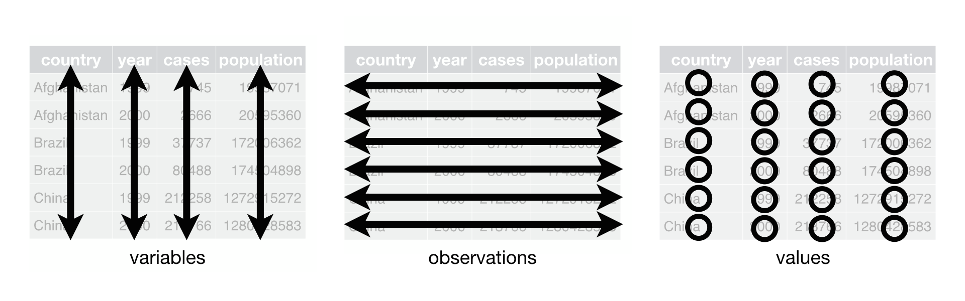
2.2.1 Values, variables, and observations

“A dataset is a collection of values, usually either numbers (if quantitative) or strings (if qualitative). Values are organized in two ways. Every value belongs to a variable and an observation.”

Source: Wickham (2014, p. 3)

Terminology:

• Value: A single element within some data structure (e.g., vector, list)
• Variables: “A variable contains all values that measure the same underlying attribute (like height, temperature, duration) across units”
• Observations: “An observation contains all values measured on the same unit (e.g., corporation-year) across attributes (variables)”
  • e.g., unit is corporation-year and one observation contains values of revenue and expense variables for Google for the 2021 fiscal year

Example: Describing data semantics [revisited]

• The experimental design data has 3 variables:
  • person, with 3 possible values (John Smith, Mary Johnson, Jane Doe)
  • treatment, with 2 possible values (treatment_a, treatment_b)
  • result, with 6 possible values (one of which is a missing value)
• Since measurements were taken for each person for each experiment, there are 6 observations:
  • 3 people x 2 treatments = 6 observations
  • For each observation, the same attribute (result) was measured
• There is a total of 18 values:
  • 3 variables x 6 observations = 18 values

2.3 Unit of analysis

unit of analysis [my term, not Wickham’s]:

• What each row represents in a dataset (referring to the physical layout of the dataset).

Examples of different units of analysis:

• if each row represents a student, you have student-level data
• if each row represents a student-course, you have student-course level data
• if each row represents an organization-year, you have organization-year level data

Questions:

• What does each row represent in the data frame object structure_a?

structure_a
#> # A tibble: 3 × 3
#>   name         treatment_a treatment_b
#>   <chr>              <dbl>       <dbl>
#> 1 John Smith            NA           2
#> 2 Jane Doe              16          11
#> 3 Mary Johnson           3           1

• What does each row represent in the data frame object structure_b?

structure_b
#> # A tibble: 2 × 4
#>   treatment   `John Smith` `Jane Doe` `Mary Johnson`
#>   <chr>              <dbl>      <dbl>          <dbl>
#> 1 treatment_a           NA         16              3
#> 2 treatment_b            2         11              1

• What does each row represent in the data frame object ipeds_hc_temp?

  • Below we load data on 12-month enrollment headcount for 2015-16 academic year from the Integrated Postsecondary Education Data System (IPEDS)

ipeds_hc_temp <- read_dta(file="https://github.com/ozanj/rclass/raw/master/data/ipeds/effy/ey15-16_hc.dta", encoding=NULL) %>% 
  select(unitid,lstudy,efytotlt) %>% arrange(unitid,lstudy)

ipeds_hc_temp
#> # A tibble: 15,726 × 3
#>    unitid lstudy                efytotlt
#>     <dbl> <dbl+lbl>                <dbl>
#>  1 100654   1 [Undergraduate]       4865
#>  2 100654   3 [Graduate]            1292
#>  3 100654 999 [Generated total]     6157
#>  4 100663   1 [Undergraduate]      13440
#>  5 100663   3 [Graduate]            8114
#>  6 100663 999 [Generated total]    21554
#>  7 100690   1 [Undergraduate]        415
#>  8 100690   3 [Graduate]             415
#>  9 100690 999 [Generated total]      830
#> 10 100706   1 [Undergraduate]       6994
#> # ℹ 15,716 more rows
#show variable labels and value labels
#ipeds_hc_temp %>% var_label()
#ipeds_hc_temp %>% val_labels()

#print a few obs, with value labels rather than variable values
ipeds_hc_temp %>% head(n=10) %>% as_factor()
#> # A tibble: 10 × 3
#>    unitid lstudy          efytotlt
#>     <dbl> <fct>              <dbl>
#>  1 100654 Undergraduate       4865
#>  2 100654 Graduate            1292
#>  3 100654 Generated total     6157
#>  4 100663 Undergraduate      13440
#>  5 100663 Graduate            8114
#>  6 100663 Generated total    21554
#>  7 100690 Undergraduate        415
#>  8 100690 Graduate             415
#>  9 100690 Generated total      830
#> 10 100706 Undergraduate       6994

2.3.1 Which variable(s) uniquely identify rows in a data frame

Identifying which combination of variables uniquely identifies rows in a data frame helps you identify the “unit of analysis” and understand the “structure” of your dataset

• Said differently: for each value of this variable (or combination of variables), there is only one row
• Very important for reshaping/tidying data (this week) and very important for joining/merging data frames (next week)
• Sometimes a codebook will explicitly tell you which vars uniquely identify rows
• Sometimes you have to figure this out through investigation
  • focus on ID variables and categorical variables that identify what each row represents; not continuous numeric variables like total_enrollment or family_income

Task: Let’s try to identify the variable(s) that uniquely identify rows in ipeds_hc_temp

• Multiple ways of doing this
• I’ll give you some code for one approach; just try to follow along and understand

names(ipeds_hc_temp)
#> [1] "unitid"   "lstudy"   "efytotlt"
ipeds_hc_temp %>% head(n=10)
#> # A tibble: 10 × 3
#>    unitid lstudy                efytotlt
#>     <dbl> <dbl+lbl>                <dbl>
#>  1 100654   1 [Undergraduate]       4865
#>  2 100654   3 [Graduate]            1292
#>  3 100654 999 [Generated total]     6157
#>  4 100663   1 [Undergraduate]      13440
#>  5 100663   3 [Graduate]            8114
#>  6 100663 999 [Generated total]    21554
#>  7 100690   1 [Undergraduate]        415
#>  8 100690   3 [Graduate]             415
#>  9 100690 999 [Generated total]      830
#> 10 100706   1 [Undergraduate]       6994

First, Let’s investigate whether the ID variable unitid uniquely identifies rows in data frame ipeds_hc_temp

• I’ll annotate code for each step

ipeds_hc_temp %>% # start with data frame object ipeds_hc_temp
  group_by(unitid) %>% # group by unitid
  summarise(n_per_group=n()) %>% # create measure of number of obs per group
  ungroup %>% # ungroup (otherwise frequency table [next step] created) separately for each group (i.e., separate frequency table for each value of unitid)
  count(n_per_group) # frequency of number of observations per group
#> # A tibble: 2 × 2
#>   n_per_group     n
#>         <int> <int>
#> 1           2  5127
#> 2           3  1824

What does above output tell us?

• There are 5,127 values of unitid that have 2 rows for that value of unitid
• There are 1,824 values of unitid that have 3 rows for that value of unitid
• Note: 2*5127+3*1824== 15,726 which is the number of observations in ipeds_hc_temp
• Conclusion: the variable unitid does not uniquely identify rows in the data frame ipeds_hc_temp

Second, Let’s investigate whether the combination of unitid and lstudy uniquely identifies rows in data frame ipeds_hc_temp.

ipeds_hc_temp %>% # start with data frame object ipeds_hc_temp
  group_by(unitid,lstudy) %>% # group by unitid and lstudy
  summarise(n_per_group=n()) %>% # create measure of number of obs per group
  ungroup %>% # ungroup (otherwise frequency table [next step] created) separately for each group (i.e., separate frequency table for each value of unitid)
  count(n_per_group) # frequency of number of observations per group
#> `summarise()` has grouped output by 'unitid'. You can override using the
#> `.groups` argument.
#> # A tibble: 1 × 2
#>   n_per_group     n
#>         <int> <int>
#> 1           1 15726

What does above output tell us?

• There is 1 row each unique combination of unitid and lstudy
• Conclusion: the variables unitid and lstudy uniquely identify rows in the data frame ipeds_hc_temp

3 Tidy vs. untidy data

3.1 Defining tidy data

“Tidy data is a standard way of mapping the meaning of a dataset to its structure.”

Source: Wickham (2014, p. 4)

Tidy data always follow these 3 interrelated rules:

1. Each variable must have its own column
2. Each observation must have its own row
3. Each value must have its own cell

Example: Representing data in tidy form

Tidy data: `table1` from the `tidyr` package

country	year	cases	population
Afghanistan	1999	745	19987071
Afghanistan	2000	2666	20595360
Brazil	1999	37737	172006362
Brazil	2000	80488	174504898
China	1999	212258	1272915272
China	2000	213766	1280428583

This table shows the same data from earlier, but now the data is in tidy form because it satisfies the 3 rules:

1. All 4 variables (country, year, cases, population) have its own column
2. All 6 observations (combination of country-year) have its own row
3. All 24 values have its own cell in the table

3.2 Diagnosing untidy data

Untidy data is any data that do not fully follow the 3 rules of tidy data defined previously.

Example: Tidy vs. untidy data

Tidy data: `table1` from the `tidyr` package

country	year	cases	population
Afghanistan	1999	745	19987071
Afghanistan	2000	2666	20595360
Brazil	1999	37737	172006362
Brazil	2000	80488	174504898
China	1999	212258	1272915272
China	2000	213766	1280428583

Untidy data: `table2` from the `tidyr` package

country	year	type	count
Afghanistan	1999	cases	745
Afghanistan	1999	population	19987071
Afghanistan	2000	cases	2666
Afghanistan	2000	population	20595360
Brazil	1999	cases	37737
Brazil	1999	population	172006362
Brazil	2000	cases	80488
Brazil	2000	population	174504898
China	1999	cases	212258
China	1999	population	1272915272
China	2000	cases	213766
China	2000	population	1280428583

The above tables show the same data, but table1 is in tidy form while table2 is untidy because it does not fully follow the 3 rules. Let’s diagnose the problems with table2 by answering these questions:

1. Does each variable have its own column?
   • If not, how does the dataset violate this principle?
   • What should the variables be?
2. Does each observation have its own row?
   • If not, how does the dataset violate this principle?
   • What does each row actually represent?
   • What should each row represent?
3. Does each value have its own cell?
   • If not, how does the dataset violate this principle?

Solutions

1. Does each variable have its own column? No
   • If not, how does the dataset violate this principle? cases and population should be two different variables because they are different attributes, but in table2 these two attributes are recorded in the column type and the associated value for each type is recorded in the column count.
   • What should the variables be? country, year, cases, population
2. Does each observation have its own row? No
   • If not, how does the dataset violate this principle? There is one observation for each country-year-type. But the values of type (cases, population) represent attributes of a unit, which should be represented by distinct variables rather than rows. So table2 has two rows per observation but it should have one row per observation.
   • What does each row actually represent? country-year-type
   • What should each row represent? country-year
3. Does each value have its own cell? Yes
   • If not, how does the dataset violate this principle?

3.3 Common types of untidy data

Tidy data can only have one organizational structure, while untidy data can come in various different forms. It is important to identify the most common types of untidy data, so that we can develop solutions for each.

Below are some of the common problems of untidy data.

3.3.1 Column headers are values, not variable names

`table4b` from the `tidyr` package

country	1999	2000
Afghanistan	19987071	20595360
Brazil	172006362	174504898
China	1272915272	1280428583

Here, 1999 and 2000 are not names of variables, but values of a variable (i.e., year). This form results in:

• A single variable spreading over multiple columns (both the last 2 columns contain values of country population)
• A single row containing multiple observations (e.g., population in 1999 Afghanistan and population in 2000 Afghanistan should be different observations)

3.3.2 Multiple variables are stored in one column

`table2` from the `tidyr` package

country	year	type	count
Afghanistan	1999	cases	745
Afghanistan	1999	population	19987071
Afghanistan	2000	cases	2666
Afghanistan	2000	population	20595360
Brazil	1999	cases	37737
Brazil	1999	population	172006362
Brazil	2000	cases	80488
Brazil	2000	population	174504898
China	1999	cases	212258
China	1999	population	1272915272
China	2000	cases	213766
China	2000	population	1280428583

cases and population are separate variables, but are stored here in the same column. This form results in:

• An observation being scattered across multiple rows (e.g., 1999 Afghanistan data should be a single observation/row)
• The values of a column not sharing the same units (the count column contains both number of cases and number of people)

3.3.3 Column contains data from two variables

`table3` from the `tidyr` package

country	year	rate
Afghanistan	1999	745/19987071
Afghanistan	2000	2666/20595360
Brazil	1999	37737/172006362
Brazil	2000	80488/174504898
China	1999	212258/1272915272
China	2000	213766/1280428583

745 and 19987071 in the rate column belong in separate columns.

3.3.4 Single variable stored in multiple columns

`table5` from the `tidyr` package

country	century	year	rate
Afghanistan	19	99	745/19987071
Afghanistan	20	00	2666/20595360
Brazil	19	99	37737/172006362
Brazil	20	00	80488/174504898
China	19	99	212258/1272915272
China	20	00	213766/1280428583

The values in century and year should be combined to form a 4-digit year variable.

4 Tidying untidy data

Approach the task of “tidying” data – or more generally, the task of “reshaping” data – as a two-step process

1. Conceptual task of understanding how the data are organized and how the data should be organized (in some order):
   • Define these concepts for your dataset
     • variables: what variables should the resulting dataset have
     • observations: each observation should represent what in the resulting dataset
   • How is the dataset currently structured (columns represent what, rows represent what)
     • which rules of tidy data are violated; why?
   • write out on a piece of scratch paper what the tidy dataset should look like
2. Technical task of writing the code that reshapes/transforms the dataset from untidy to tidy
   • pivot_longer() function reshapes data from “wide to long”
     • e.g., your dataset has separate variables for each year, but you should have one variable “year” that has rows for each value of year
   • pivot_wider() function reshapes data from “long to wide”

4.1 Reshaping wide to long: pivot_longer()

Now that we have a better understanding of the differences between tidy and untidy data, let’s practice reshaping our data. In the next two sections we are introducing the pivot_longer() and pivot_wider() functions to reshape our data.

The pivot_longer() function:

?pivot_longer

# SYNTAX AND DEFAULT VALUES
pivot_longer(data, cols, names_to = "name", names_prefix = NULL,
             names_sep = NULL, names_pattern = NULL, names_ptypes = list(),
             names_repair = "check_unique", values_to = "value",
             values_drop_na = FALSE, values_ptypes = list())

• Function: “lengthens” data, increasing the number of rows and decreasing the number of columns
• Arguments (selected):
  • data: Dataframe to pivot
  • cols: Columns to pivot into longer format
  • names_to: Name of the column to create from the data stored in the column names of data
  • values_to: Name of the column to create from the data stored in cell values
  • names_sep: If names_to contains multiple values, these arguments control how the column name is broken up.

Example: Tidying table4b (reshaping wide to long)

As seen above, the first common reason for untidy data is that some of the column names are not names of variables, but values of a variable (e.g., table4a, table4b):

country	1999	2000
Afghanistan	19987071	20595360
Brazil	172006362	174504898
China	1272915272	1280428583

The solution to this problem is to transform the untidy columns (which represent variable values) into rows. Thus, we want to transform table4b into something that looks like this:

country	year	population
Afghanistan	1999	19987071
Afghanistan	2000	20595360
Brazil	1999	172006362
Brazil	2000	174504898
China	1999	1272915272
China	2000	1280428583

This can be achieved using pivot_longer():

table4b
#> # A tibble: 3 × 3
#>   country         `1999`     `2000`
#>   <chr>            <dbl>      <dbl>
#> 1 Afghanistan   19987071   20595360
#> 2 Brazil       172006362  174504898
#> 3 China       1272915272 1280428583

table4b %>%
  pivot_longer(
    cols = c('1999', '2000'),  # pivot `1999` and `2000` columns into longer format 
    names_to = 'year',         # name of column that holds the pivoted values
    values_to = 'population'   # name of column that holds the original cell values
  )
#> # A tibble: 6 × 3
#>   country     year  population
#>   <chr>       <chr>      <dbl>
#> 1 Afghanistan 1999    19987071
#> 2 Afghanistan 2000    20595360
#> 3 Brazil      1999   172006362
#> 4 Brazil      2000   174504898
#> 5 China       1999  1272915272
#> 6 China       2000  1280428583

Example: Choosing which column not to pivot

Looking at the previous example, we could have also equivalently pivoted the table by specifying which column we want to keep unchanged:

table4b %>%
  pivot_longer(
    cols = -country,           # pivot all columns except `country`
    names_to = 'year',         # name of column that holds the pivoted values
    values_to = 'population'   # name of column that holds the original cell values
  )
#> # A tibble: 6 × 3
#>   country     year  population
#>   <chr>       <chr>      <dbl>
#> 1 Afghanistan 1999    19987071
#> 2 Afghanistan 2000    20595360
#> 3 Brazil      1999   172006362
#> 4 Brazil      2000   174504898
#> 5 China       1999  1272915272
#> 6 China       2000  1280428583

Example: Renaming pivoted columns

Sometimes, the name of the columns we want to pivot contain additional information that we want to remove before transforming to tidy data. Consider the following example where the columns all contain the prefix tot_:

nces_table1
#> # A tibble: 51 × 5
#>    state                tot_2000 tot_2010 tot_2011 tot_2012
#>    <chr>                   <dbl>    <dbl>    <dbl>    <dbl>
#>  1 Alabama                728351   730427   731556   740475
#>  2 Alaska                 105333   132104   131166   131483
#>  3 Arizona                877696  1067210  1024454   990378
#>  4 Arkansas               449959   482114   483114   486157
#>  5 California            6050753  6169427  6202862  6178788
#>  6 Colorado               724349   842864   853610   863121
#>  7 Connecticut            562179   552919   543883   549295
#>  8 Delaware               114676   128342   128470   127791
#>  9 District of Columbia    68380    71263    72329    75411
#> 10 Florida               2434755  2641555  2668037  2691881
#> # ℹ 41 more rows

If we pivot the table as is, we can see the tot_ prefixes appearing in the year column:

nces_table1 %>%
  pivot_longer(
    cols = -state,                # pivot all columns except `state`
    names_to = 'year',            # name of column that holds the pivoted values
    values_to = 'total_students'  # name of column that holds the original cell values
  )
#> # A tibble: 204 × 3
#>    state   year     total_students
#>    <chr>   <chr>             <dbl>
#>  1 Alabama tot_2000         728351
#>  2 Alabama tot_2010         730427
#>  3 Alabama tot_2011         731556
#>  4 Alabama tot_2012         740475
#>  5 Alaska  tot_2000         105333
#>  6 Alaska  tot_2010         132104
#>  7 Alaska  tot_2011         131166
#>  8 Alaska  tot_2012         131483
#>  9 Arizona tot_2000         877696
#> 10 Arizona tot_2010        1067210
#> # ℹ 194 more rows

To fix this, we can specify the names_prefix argument in pivot_longer() to match and remove the part of the names that we don’t want to keep:

nces_table1 %>%
  pivot_longer(
    cols = -state,                
    names_to = 'year',            
    names_prefix = 'tot_',        # rename pivoted values by striping the prefix 'tot_'
    values_to = 'total_students'
  )
#> # A tibble: 204 × 3
#>    state   year  total_students
#>    <chr>   <chr>          <dbl>
#>  1 Alabama 2000          728351
#>  2 Alabama 2010          730427
#>  3 Alabama 2011          731556
#>  4 Alabama 2012          740475
#>  5 Alaska  2000          105333
#>  6 Alaska  2010          132104
#>  7 Alaska  2011          131166
#>  8 Alaska  2012          131483
#>  9 Arizona 2000          877696
#> 10 Arizona 2010         1067210
#> # ℹ 194 more rows

Example: Pivoting columns by name pattern

Consider the following example where the columns we want to reshape belongs to multiple variables. As seen, the 4 columns starting with tot_ shows total student enrollment while the 4 columns starting with frl_ shows number of students on free/reduced lunch:

nces_table2
#> # A tibble: 51 × 9
#>    state tot_2000 tot_2010 tot_2011 tot_2012 frl_2000 frl_2010 frl_2011 frl_2012
#>    <chr>    <dbl>    <dbl>    <dbl>    <dbl>    <dbl>    <dbl>    <dbl>    <dbl>
#>  1 Alab…   728351   730427   731556   740475   335143   402386  420447    429604
#>  2 Alas…   105333   132104   131166   131483    32468    50701   53238     53082
#>  3 Ariz…   877696  1067210  1024454   990378   274277   482044  511885    514193
#>  4 Arka…   449959   482114   483114   486157   205058   291608  294324    298573
#>  5 Cali…  6050753  6169427  6202862  6178788  2820611  3335885 3353964.  3478407
#>  6 Colo…   724349   842864   853610   863121   195148   336426  348896    358876
#>  7 Conn…   562179   552919   543883   549295   143030   190554  194339    201085
#>  8 Dela…   114676   128342   128470   127791    37766    61564   62774     66413
#>  9 Dist…    68380    71263    72329    75411    47839    52027   45199     46416
#> 10 Flor…  2434755  2641555  2668037  2691881  1079009  1479519 1535670   1576379
#> # ℹ 41 more rows

Applying the same approach we used for nces_table1 doesn’t give us the structure we want

nces_table2 %>%
  pivot_longer(
    cols = -state,                
    names_to = 'year',            
    names_prefix = 'tot_',        # rename pivoted values by striping the prefix 'tot_'
    values_to = 'total_students'
  )
#> # A tibble: 408 × 3
#>    state   year     total_students
#>    <chr>   <chr>             <dbl>
#>  1 Alabama 2000             728351
#>  2 Alabama 2010             730427
#>  3 Alabama 2011             731556
#>  4 Alabama 2012             740475
#>  5 Alabama frl_2000         335143
#>  6 Alabama frl_2010         402386
#>  7 Alabama frl_2011         420447
#>  8 Alabama frl_2012         429604
#>  9 Alaska  2000             105333
#> 10 Alaska  2010             132104
#> # ℹ 398 more rows

The goal is to keep enrollment and lunch data in separate columns and only pivot the years part. To do this, we can provide a character vector (instead of the usual string) for names_to and additionally specify the names_sep argument.

Here, we copy the full description of the names_to and names_sep arguments from the pivot_longer() helpfile

• names_sep: If names_to contains multiple values, these arguments control how the column name is broken up.
• names_to A string specifying the name of the column to create from the data stored in the column names of data.
  • can be a character vector, creating multiple columns, if names_sep or names_pattern is provided. In this case, there are two special values you can take advantage of:
    • NA will discard that component of the name.
    • .value indicates that component of the name defines the name of the column containing the cell values, overriding values_to.

How we will use these arguments to reshape nces_table2:

• names_sep specifies the separator to use to separate the column names to 2 parts (e.g., the tot/frl measure part and the years part).
• names_to Then, we can specify how we want to treat each part inside the names_to vector:
  • Use .value to indicate the part that we want to retain as separate columns (this replaces the need for the values_to argument)
  • Provide a string to indicate the part to pivot to rows, where the string you provide will become the name of that column (like how we’d normally specify names_to)

nces_table2 %>% head(n=5)
#> # A tibble: 5 × 9
#>   state  tot_2000 tot_2010 tot_2011 tot_2012 frl_2000 frl_2010 frl_2011 frl_2012
#>   <chr>     <dbl>    <dbl>    <dbl>    <dbl>    <dbl>    <dbl>    <dbl>    <dbl>
#> 1 Alaba…   728351   730427   731556   740475   335143   402386  420447    429604
#> 2 Alaska   105333   132104   131166   131483    32468    50701   53238     53082
#> 3 Arizo…   877696  1067210  1024454   990378   274277   482044  511885    514193
#> 4 Arkan…   449959   482114   483114   486157   205058   291608  294324    298573
#> 5 Calif…  6050753  6169427  6202862  6178788  2820611  3335885 3353964.  3478407

nces_table2 %>%
  pivot_longer(
    -state,                          # pivot all columns except `state`
    names_sep = '_',                  # use '_' as column name separator    
    names_to = c('.value', 'year')  # keep `tot` & `frl` as separate columns, pivot year values
  )
#> # A tibble: 204 × 4
#>    state   year      tot    frl
#>    <chr>   <chr>   <dbl>  <dbl>
#>  1 Alabama 2000   728351 335143
#>  2 Alabama 2010   730427 402386
#>  3 Alabama 2011   731556 420447
#>  4 Alabama 2012   740475 429604
#>  5 Alaska  2000   105333  32468
#>  6 Alaska  2010   132104  50701
#>  7 Alaska  2011   131166  53238
#>  8 Alaska  2012   131483  53082
#>  9 Arizona 2000   877696 274277
#> 10 Arizona 2010  1067210 482044
#> # ℹ 194 more rows

Note the difference if we used .value as the second element in names_to:

nces_table2 %>%
  pivot_longer(
    -state,
    names_to = c('measure', '.value'),  # pivot `tot`/`frl`, keep years as separate columns
    names_sep = '_'
  )
#> # A tibble: 102 × 6
#>    state      measure  `2000`  `2010`   `2011`  `2012`
#>    <chr>      <chr>     <dbl>   <dbl>    <dbl>   <dbl>
#>  1 Alabama    tot      728351  730427  731556   740475
#>  2 Alabama    frl      335143  402386  420447   429604
#>  3 Alaska     tot      105333  132104  131166   131483
#>  4 Alaska     frl       32468   50701   53238    53082
#>  5 Arizona    tot      877696 1067210 1024454   990378
#>  6 Arizona    frl      274277  482044  511885   514193
#>  7 Arkansas   tot      449959  482114  483114   486157
#>  8 Arkansas   frl      205058  291608  294324   298573
#>  9 California tot     6050753 6169427 6202862  6178788
#> 10 California frl     2820611 3335885 3353964. 3478407
#> # ℹ 92 more rows

Practical example of using the pivot_longer() function in the Appendix

4.2 Reshaping long to wide: pivot_wider()

The pivot_wider() function:

?pivot_wider

# SYNTAX AND DEFAULT VALUES
pivot_wider(data, id_cols = NULL, names_from = name,
            names_prefix = "", names_sep = "_", names_repair = "check_unique",
            values_from = value, values_fill = NULL, values_fn = NULL)

• Function: “widens” data, increasing the number of columns and decreasing the number of rows
• Arguments:
  • data: Dataframe to pivot
  • names_from: Column(s) to get the name of the output column
  • values_from: Column(s) to get the cell values from

Example: Tidying table2 (reshaping long to wide)

As seen previously, the second common reason for untidy data is that multiple variables are stored in one column (e.g., table2):

• An observation is scattered across multiple rows
• One column identifies variable type (e.g., type) and another column contains the values for each variable (e.g., count)

country	year	type	count
Afghanistan	1999	cases	745
Afghanistan	1999	population	19987071
Afghanistan	2000	cases	2666
Afghanistan	2000	population	20595360
Brazil	1999	cases	37737
Brazil	1999	population	172006362
Brazil	2000	cases	80488
Brazil	2000	population	174504898
China	1999	cases	212258
China	1999	population	1272915272
China	2000	cases	213766
China	2000	population	1280428583

This sort of data structure is very common “in the wild” (e.g., in data that you download), and it is up to you to tidy it before analyses.

The solution to this problem is to transform the untidy rows (which represent different variables) into columns. Thus, we want to transform table2 into something that looks like this:

country	year	cases	population
Afghanistan	1999	745	19987071
Afghanistan	2000	2666	20595360
Brazil	1999	37737	172006362
Brazil	2000	80488	174504898
China	1999	212258	1272915272
China	2000	213766	1280428583

This can be achieved using pivot_wider():

table2
#> # A tibble: 12 × 4
#>    country      year type            count
#>    <chr>       <dbl> <chr>           <dbl>
#>  1 Afghanistan  1999 cases             745
#>  2 Afghanistan  1999 population   19987071
#>  3 Afghanistan  2000 cases            2666
#>  4 Afghanistan  2000 population   20595360
#>  5 Brazil       1999 cases           37737
#>  6 Brazil       1999 population  172006362
#>  7 Brazil       2000 cases           80488
#>  8 Brazil       2000 population  174504898
#>  9 China        1999 cases          212258
#> 10 China        1999 population 1272915272
#> 11 China        2000 cases          213766
#> 12 China        2000 population 1280428583

table2 %>%
  pivot_wider(
    names_from = type,   # values in `type` become variable names
    values_from = count  # values in `count` become values in the new `cases` and `population` cols
  )
#> # A tibble: 6 × 4
#>   country      year  cases population
#>   <chr>       <dbl>  <dbl>      <dbl>
#> 1 Afghanistan  1999    745   19987071
#> 2 Afghanistan  2000   2666   20595360
#> 3 Brazil       1999  37737  172006362
#> 4 Brazil       2000  80488  174504898
#> 5 China        1999 212258 1272915272
#> 6 China        2000 213766 1280428583

Example: Pivoting with multiple value variables

Sometimes, we want to spread a dataset that contains multiple value variables. Consider the following example where there are separate enrollment variables for total, men, and women:

ipeds_table1
#> # A tibble: 15,726 × 5
#>    unitid efytotlt efytotlm efytotlw level
#>     <dbl>    <dbl>    <dbl>    <dbl> <chr>
#>  1 100654     6157     2646     3511 all  
#>  2 100654     4865     2258     2607 ug   
#>  3 100654     1292      388      904 grad 
#>  4 100663    21554     8383    13171 all  
#>  5 100663    13440     5552     7888 ug   
#>  6 100663     8114     2831     5283 grad 
#>  7 100690      830      337      493 all  
#>  8 100690      415      177      238 ug   
#>  9 100690      415      160      255 grad 
#> 10 100706     9206     5194     4012 all  
#> # ℹ 15,716 more rows

The goal is to turn the values in levels into columns - but which of the enrollment variables should be used as the values for the new columns? The solution is to create columns for each of the enrollment variables:

ipeds_table1 %>%
  pivot_wider(
    names_from = level,
    values_from = c(efytotlt, efytotlm, efytotlw)
  )
#> # A tibble: 6,951 × 10
#>    unitid efytotlt_all efytotlt_ug efytotlt_grad efytotlm_all efytotlm_ug
#>     <dbl>        <dbl>       <dbl>         <dbl>        <dbl>       <dbl>
#>  1 100654         6157        4865          1292         2646        2258
#>  2 100663        21554       13440          8114         8383        5552
#>  3 100690          830         415           415          337         177
#>  4 100706         9206        6994          2212         5194        3983
#>  5 100724         6101        5373           728         2321        2105
#>  6 100751        41507       35199          6308        18526       15946
#>  7 100760         2379        2379            NA         1027        1027
#>  8 100812         4124        4124            NA         1478        1478
#>  9 100830         5996        5072           924         2158        1847
#> 10 100858        29237       22953          6284        14893       11871
#> # ℹ 6,941 more rows
#> # ℹ 4 more variables: efytotlm_grad <dbl>, efytotlw_all <dbl>,
#> #   efytotlw_ug <dbl>, efytotlw_grad <dbl>

Practical example of using the pivot_wider() function in the Appendix

5 Missing values

5.1 Explicit vs. Implicit missing values

There are two types of missing values:

• Explicit missing values: variable has the value NA for a particular row
• Implicit missing values: the row is simply not present in the data

Example: Identifying explicit and implicit missing values

Consider the following dataset, which shows stock return for each year and quarter for some hypothetical company:

year	qtr	return
2015	1	1.88
2015	2	0.59
2015	3	0.35
2015	4	NA
2016	2	0.92
2016	3	0.17
2016	4	2.66

The variable return has:

• 1 explicit missing value: There is an NA in the 4th quarter of 2015
• 1 implicit missing value: Data for the 1st quarter of 2016 simply does not exist

Practical example of identifying explicit and implicit missing values in the Appendix

5.2 Making implicit missing values explicit

An implicit missing value is the result of a row not existing. In order to make an implicit missing value explicit, we need to make the non-existent row exist. This can be done using the complete() function within tidyr.

The complete() function:

?complete

# SYNTAX AND DEFAULT VALUES
complete(data, ..., fill = list())

• Function: Turns implicit missing values into explicit missing values
• Arguments:
  • data: A dataframe
  • ...: Variables to expand on
• Returns: A dataframe object that has all unique combinations of the specified variables, including those not found in the original dataframe

Example: Making implicit missing values explicit

Recall the stocks dataset from the previous example. There was 1 implicit missing value for the 1st quarter of 2016 - that row simply did not exist.

If we want to turn that into an explicit missing value, then we need the row for the 1st quarter of 2016 to exist. The result would look like this:

year	qtr	return
2015	1	1.88
2015	2	0.59
2015	3	0.35
2015	4	NA
2016	1	NA
2016	2	0.92
2016	3	0.17
2016	4	2.66

We can achieve this by using the complete() function:

stocks
#> # A tibble: 7 × 3
#>    year   qtr return
#>   <dbl> <dbl>  <dbl>
#> 1  2015     1   1.88
#> 2  2015     2   0.59
#> 3  2015     3   0.35
#> 4  2015     4  NA   
#> 5  2016     2   0.92
#> 6  2016     3   0.17
#> 7  2016     4   2.66

stocks %>%
  complete(year, qtr)
#> # A tibble: 8 × 3
#>    year   qtr return
#>   <dbl> <dbl>  <dbl>
#> 1  2015     1   1.88
#> 2  2015     2   0.59
#> 3  2015     3   0.35
#> 4  2015     4  NA   
#> 5  2016     1  NA   
#> 6  2016     2   0.92
#> 7  2016     3   0.17
#> 8  2016     4   2.66

Should you make implicit missing values explicit?

• No clear-cut answer - it depends on many context-specific things about your project
• The important thing is to be aware of the presence of implicit missing values (both in the “input” datasets you read in and the datasets you create from the inputs) and be purposeful about how you deal with implicit missing values
• Recommendation for the stage of creating analysis datasets from input data:
  • If you feel unsure about making implicit values explicit, then make them explicit
  • This forces you to be more fully aware of patterns of missing data and helps you avoid careless mistakes down the road
  • After making implicit missing values explicit, you can drop these rows once you are sure you don’t need them

Practical example of using the complete() function in the Appendix

5.3 Reshaping long to wide: missing values

Let’s take a look at what happens with missing values when we reshape from long to wide. Recall the stocks dataset from the earlier example, where we have 1 explicit missing value (2015 4th quarter) and 1 implicit missing value (2016 1st quarter):

year	qtr	return
2015	1	1.88
2015	2	0.59
2015	3	0.35
2015	4	NA
2016	2	0.92
2016	3	0.17
2016	4	2.66

When we reshape it from long to wide using pivot_wider(), notice that both implicit and explicit missing values appear as NA. In other words, implicit missing values are automatically turned into explicit missing values. Therefore, there is no need to use complete() prior to pivoting.

stocks %>% pivot_wider(
  names_from = qtr,
  values_from = return
)

year	1	2	3	4
2015	1.88	0.59	0.35	NA
2016	NA	0.92	0.17	2.66

Note that we can no longer tell whether the NAs used to be implicit or explicit missing values, as they are now all explicit. One way to be able to distinguish between them is by specifying the values_fill argument when calling pivot_wider(). This will fill in the previously implicit values with any value of your choice, meaning any NA you see after reshaping must be from the previously explicit missing values. In other words, explicit missing values stay explicit while implicit missing values are filled.

stocks %>% pivot_wider(
  names_from = qtr,
  values_from = return,
  values_fill = list(return = -99)
)

year	1	2	3	4
2015	1.88	0.59	0.35	NA
2016	-99.00	0.92	0.17	2.66

6 Appendix

6.1 Student exercise: Real-world example of wide to long

[In the task I present below, you have the option to work through the solution I have created or try doing it on your own before you look at solution]

The following dataset is drawn from Table 204.10 of the NCES Digest for Education Statistics.

• The table shows change over time in the number and percentage of K-12 students on free/reduced lunch for selected years.
• LINK to website with data

#Let's take a look at the data (we read in the data in the wide vs long section)
glimpse(nces_table)
#> Rows: 51
#> Columns: 13
#> $ state      <chr> "Alabama", "Alaska", "Arizona", "Arkansas", "California", "…
#> $ tot_2000   <dbl> 728351, 105333, 877696, 449959, 6050753, 724349, 562179, 11…
#> $ tot_2010   <dbl> 730427, 132104, 1067210, 482114, 6169427, 842864, 552919, 1…
#> $ tot_2011   <dbl> 731556, 131166, 1024454, 483114, 6202862, 853610, 543883, 1…
#> $ tot_2012   <dbl> 740475, 131483, 990378, 486157, 6178788, 863121, 549295, 12…
#> $ frl_2000   <dbl> 335143, 32468, 274277, 205058, 2820611, 195148, 143030, 377…
#> $ frl_2010   <dbl> 402386, 50701, 482044, 291608, 3335885, 336426, 190554, 615…
#> $ frl_2011   <dbl> 420447.00, 53238.00, 511885.00, 294324.00, 3353963.72, 3488…
#> $ frl_2012   <dbl> 429604, 53082, 514193, 298573, 3478407, 358876, 201085, 664…
#> $ p_frl_2000 <dbl> 46.01394, 30.82415, 31.24966, 45.57260, 46.61587, 26.94116,…
#> $ p_frl_2010 <dbl> 55.08915, 38.37961, 45.16862, 60.48528, 54.07123, 39.91462,…
#> $ p_frl_2011 <dbl> 57.47298, 40.58826, 49.96662, 60.92227, 54.07123, 40.87300,…
#> $ p_frl_2012 <dbl> 58.01735, 40.37176, 51.91886, 61.41493, 56.29594, 41.57887,…

#Create smaller version of data frame for purpose of student exercise
total<- nces_table %>% 
  select(state,p_frl_2000,p_frl_2010,p_frl_2011,p_frl_2012)
head(total)
#> # A tibble: 6 × 5
#>   state      p_frl_2000 p_frl_2010 p_frl_2011 p_frl_2012
#>   <chr>           <dbl>      <dbl>      <dbl>      <dbl>
#> 1 Alabama          46.0       55.1       57.5       58.0
#> 2 Alaska           30.8       38.4       40.6       40.4
#> 3 Arizona          31.2       45.2       50.0       51.9
#> 4 Arkansas         45.6       60.5       60.9       61.4
#> 5 California       46.6       54.1       54.1       56.3
#> 6 Colorado         26.9       39.9       40.9       41.6

Task (using the data frame total):

1. Diagnose the problem with the data frame total
2. Sketch out what the tidy data should look like
   
3. Transform untidy to tidy. hint: use names_prefix

Solution to student exercise:

1. Diagnose the problem with the data frame total
   • Column names p_frl_2000, p_frl_2010, etc. are not variables; rather they refer to values of the variable year
   • Currently each observation represents a state with separate number of students on FRL variables for each year.
   • Each observation should be a state-year, with only one variable for FRL
2. Sketch out what the tidy data should look like
   
3. Transform untidy to tidy
   • names of the set of columns that represent values, not variables in your untidy data
     • p_frl_2000,p_frl_2010,p_frl_2011,p_frl_2012
   • names_to : variable name you will assign to columns you are gathering from the untidy data
     • This var doesn’t yet exist in untidy data, but will be a variable name in the tidy data
     • In this example, it’s year
   • values_to: The name of the variable that will contain values in the tidy dataset you create and whose values are spread across multiple columns in the untidy dataset
     • This var doesn’t yet exist in untidy data, but will be a variable name in the tidy data
     • in this example, the value variable is frl_students

total %>%
  pivot_longer(
    cols = starts_with("p_frl_"),
    names_to = "year",
    names_prefix = ("p_frl_"),
    values_to = "pct_frl"
  )
#> # A tibble: 204 × 3
#>    state   year  pct_frl
#>    <chr>   <chr>   <dbl>
#>  1 Alabama 2000     46.0
#>  2 Alabama 2010     55.1
#>  3 Alabama 2011     57.5
#>  4 Alabama 2012     58.0
#>  5 Alaska  2000     30.8
#>  6 Alaska  2010     38.4
#>  7 Alaska  2011     40.6
#>  8 Alaska  2012     40.4
#>  9 Arizona 2000     31.2
#> 10 Arizona 2010     45.2
#> # ℹ 194 more rows

6.2 Student exercise: real-world example of reshaping long to wide

[In the task I present below, you have the option to work through the solution I have created or try doing it on your own before you look at solution]

The Integrated Postsecondary Education Data System (IPEDS) collects data on colleges and universities

• Below we load IPEDS data on 12-month enrollment headcount for 2015-16 academic year

#load these libraries if you haven't already
#library(haven)
#library(labelled)
# ipeds_table <- read_dta(file="https://github.com/ozanj/rclass/raw/master/data/ipeds/effy/ey15-16_hc.dta", encoding=NULL)

Create smaller version of dataset

#ipeds_hc <- ipeds_table %>% select(instnm,unitid,lstudy,efytotlt,efytotlm,efytotlw)
ipeds_hc <- ipeds_table %>% select(instnm,unitid,lstudy,efytotlt)

Get to know data

head(ipeds_hc)
#> # A tibble: 6 × 4
#>   instnm                              unitid lstudy                efytotlt
#>   <chr>                                <dbl> <dbl+lbl>                <dbl>
#> 1 Alabama A & M University            100654 999 [Generated total]     6157
#> 2 Alabama A & M University            100654   1 [Undergraduate]       4865
#> 3 Alabama A & M University            100654   3 [Graduate]            1292
#> 4 University of Alabama at Birmingham 100663 999 [Generated total]    21554
#> 5 University of Alabama at Birmingham 100663   1 [Undergraduate]      13440
#> 6 University of Alabama at Birmingham 100663   3 [Graduate]            8114
str(ipeds_hc)
#> tibble [15,726 × 4] (S3: tbl_df/tbl/data.frame)
#>  $ instnm  : chr [1:15726] "Alabama A & M University" "Alabama A & M University" "Alabama A & M University" "University of Alabama at Birmingham" ...
#>   ..- attr(*, "label")= chr "Institution (entity) name"
#>   ..- attr(*, "format.stata")= chr "%91s"
#>  $ unitid  : num [1:15726] 100654 100654 100654 100663 100663 ...
#>   ..- attr(*, "label")= chr "Unique identification number of the institution"
#>   ..- attr(*, "format.stata")= chr "%12.0g"
#>  $ lstudy  : dbl+lbl [1:15726] 999,   1,   3, 999,   1,   3, 999,   1,   3, 999,   ...
#>    ..@ label       : chr "Original level of study on survey form"
#>    ..@ format.stata: chr "%15.0g"
#>    ..@ labels      : Named num [1:3] 1 3 999
#>    .. ..- attr(*, "names")= chr [1:3] "Undergraduate" "Graduate" "Generated total"
#>  $ efytotlt: num [1:15726] 6157 4865 1292 21554 13440 ...
#>   ..- attr(*, "label")= chr "Grand total"
#>   ..- attr(*, "format.stata")= chr "%12.0g"
#>  - attr(*, "label")= chr "dct_s2015_is"

#Variable labels
ipeds_hc %>% var_label()
#> $instnm
#> [1] "Institution (entity) name"
#> 
#> $unitid
#> [1] "Unique identification number of the institution"
#> 
#> $lstudy
#> [1] "Original level of study on survey form"
#> 
#> $efytotlt
#> [1] "Grand total"

#Only the variable lstudy has value labels
ipeds_hc %>% select(lstudy) %>% val_labels()
#> $lstudy
#>   Undergraduate        Graduate Generated total 
#>               1               3             999

Student Task:

1. Diagnose the problem with the data frame ipeds_hc (why is it untidy?)
2. Sketch out what the tidy data should look like
   
3. Transform untidy to tidy

Solution to student task:

1. Diagnose the problem with the data frame - First, let’s investigate the data

ipeds_hc <- ipeds_hc %>% arrange(unitid, lstudy)
head(ipeds_hc, n=20)
#> # A tibble: 20 × 4
#>    instnm                              unitid lstudy                efytotlt
#>    <chr>                                <dbl> <dbl+lbl>                <dbl>
#>  1 Alabama A & M University            100654   1 [Undergraduate]       4865
#>  2 Alabama A & M University            100654   3 [Graduate]            1292
#>  3 Alabama A & M University            100654 999 [Generated total]     6157
#>  4 University of Alabama at Birmingham 100663   1 [Undergraduate]      13440
#>  5 University of Alabama at Birmingham 100663   3 [Graduate]            8114
#>  6 University of Alabama at Birmingham 100663 999 [Generated total]    21554
#>  7 Amridge University                  100690   1 [Undergraduate]        415
#>  8 Amridge University                  100690   3 [Graduate]             415
#>  9 Amridge University                  100690 999 [Generated total]      830
#> 10 University of Alabama in Huntsville 100706   1 [Undergraduate]       6994
#> 11 University of Alabama in Huntsville 100706   3 [Graduate]            2212
#> 12 University of Alabama in Huntsville 100706 999 [Generated total]     9206
#> 13 Alabama State University            100724   1 [Undergraduate]       5373
#> 14 Alabama State University            100724   3 [Graduate]             728
#> 15 Alabama State University            100724 999 [Generated total]     6101
#> 16 The University of Alabama           100751   1 [Undergraduate]      35199
#> 17 The University of Alabama           100751   3 [Graduate]            6308
#> 18 The University of Alabama           100751 999 [Generated total]    41507
#> 19 Central Alabama Community College   100760   1 [Undergraduate]       2379
#> 20 Central Alabama Community College   100760 999 [Generated total]     2379

#code to investigate what each observation represents
  #I'll break this code down next week when we talk about joining data frames
ipeds_hc %>% group_by(unitid,lstudy) %>% # group_by our candidate
  mutate(n_per_id=n()) %>% # calculate number of obs per group
  ungroup() %>% # ungroup the data
  count(n_per_id==1) # count "true that only one obs per group"
#> # A tibble: 1 × 2
#>   `n_per_id == 1`     n
#>   <lgl>           <int>
#> 1 TRUE            15726

Summary of problems with the data frame:

• In the untidy data frame, each row represents college-level_of_study
  • there are separate rows for each value of level of study (undergraduate, graduate, generated total)
  • so three rows for each college
• the values of the column lstudy represent different attributes (undergraduate, graduate, generated total)
  • each of these attributes should be its own variable

2. Sketch out what the tidy data should look like (sketch out on your own)

• What tidy data should look like:
  • Each observation (row) should be a college
  • There should be separate variables for each level of study, with each variable containing enrollment for that level of study

3. Transform untidy to tidy

• names_from. Column name in the untidy data whose values will become variable names in the tidy data that contains variable names
  • this variable name exists in the untidy data
  • in ipeds_hc the key column is lstudy; the values of lstudy, will become variable names in the tidy data
• values_from. Column name in untidy data that contains values for the new variables that will be created in the tidy data
  • this is a varname that exists in the untidy data
  • in ipeds_hc the value column is efytotlt; the values of efytotlt will become the values of the new variables in the tidy data

ipeds_hc %>% 
    pivot_wider(names_from = lstudy, values_from = efytotlt) #notice it uses the underlying data not labels
#> # A tibble: 6,951 × 5
#>    instnm                              unitid   `1`   `3` `999`
#>    <chr>                                <dbl> <dbl> <dbl> <dbl>
#>  1 Alabama A & M University            100654  4865  1292  6157
#>  2 University of Alabama at Birmingham 100663 13440  8114 21554
#>  3 Amridge University                  100690   415   415   830
#>  4 University of Alabama in Huntsville 100706  6994  2212  9206
#>  5 Alabama State University            100724  5373   728  6101
#>  6 The University of Alabama           100751 35199  6308 41507
#>  7 Central Alabama Community College   100760  2379    NA  2379
#>  8 Athens State University             100812  4124    NA  4124
#>  9 Auburn University at Montgomery     100830  5072   924  5996
#> 10 Auburn University                   100858 22953  6284 29237
#> # ℹ 6,941 more rows

Alternative solution:

Helpful to create a character version of variable lstudy prior to spreading

ipeds_hc %>% select(lstudy) %>% val_labels()
#> $lstudy
#>   Undergraduate        Graduate Generated total 
#>               1               3             999
str(ipeds_hc$lstudy)
#>  dbl+lbl [1:15726]   1,   3, 999,   1,   3, 999,   1,   3, 999,   1,   3, 9...
#>  @ label       : chr "Original level of study on survey form"
#>  @ format.stata: chr "%15.0g"
#>  @ labels      : Named num [1:3] 1 3 999
#>   ..- attr(*, "names")= chr [1:3] "Undergraduate" "Graduate" "Generated total"

ipeds_hcv2 <- ipeds_hc %>% 
  mutate(level = recode(as.integer(lstudy),
    `1` = "ug",
    `3` = "grad",
    `999` = "all")
  ) %>% select(-lstudy) # drop variable lstudy

head(ipeds_hcv2)
#> # A tibble: 6 × 4
#>   instnm                              unitid efytotlt level
#>   <chr>                                <dbl>    <dbl> <chr>
#> 1 Alabama A & M University            100654     4865 ug   
#> 2 Alabama A & M University            100654     1292 grad 
#> 3 Alabama A & M University            100654     6157 all  
#> 4 University of Alabama at Birmingham 100663    13440 ug   
#> 5 University of Alabama at Birmingham 100663     8114 grad 
#> 6 University of Alabama at Birmingham 100663    21554 all

ipeds_hcv2 %>% select(instnm,unitid,level,efytotlt) %>%
    pivot_wider(names_from = level, values_from = efytotlt) #nicer!
#> # A tibble: 6,951 × 5
#>    instnm                              unitid    ug  grad   all
#>    <chr>                                <dbl> <dbl> <dbl> <dbl>
#>  1 Alabama A & M University            100654  4865  1292  6157
#>  2 University of Alabama at Birmingham 100663 13440  8114 21554
#>  3 Amridge University                  100690   415   415   830
#>  4 University of Alabama in Huntsville 100706  6994  2212  9206
#>  5 Alabama State University            100724  5373   728  6101
#>  6 The University of Alabama           100751 35199  6308 41507
#>  7 Central Alabama Community College   100760  2379    NA  2379
#>  8 Athens State University             100812  4124    NA  4124
#>  9 Auburn University at Montgomery     100830  5072   924  5996
#> 10 Auburn University                   100858 22953  6284 29237
#> # ℹ 6,941 more rows

6.3 Missing variables example using IPEDS

This section deals with missing variables and tidying data.

But first, it is helpful to create a new version of the IPEDS enrollment dataset as follows:

• keeps observations for for-profit colleges

• keeps the following enrollment variables:

  • total enrollment
  • enrollment of students who identify as “Black or African American”

  ipeds_hc_na <- ipeds_table %>% filter(sector %in% c(3,6,9)) %>% #keep only for-profit colleges
    select(instnm,unitid,lstudy,efytotlt,efybkaam) %>% 
    mutate(level = recode(as.integer(lstudy), # create recoded version of lstudy
      `1` = "ug",
      `3` = "grad",
      `999` = "all")
    ) %>% select(instnm,unitid,level,efytotlt,efybkaam) %>% 
    arrange(unitid,desc(level))

Now, let’s print some rows

• There is one row for each college-level_of_study
• Some colleges have three rows of data (ug, grad, all)
• Colleges that don’t have any undergraduates or don’t have any graduate students only have two rows of data

ipeds_hc_na
#> # A tibble: 6,265 × 5
#>    instnm                               unitid level efytotlt efybkaam
#>    <chr>                                 <dbl> <chr>    <dbl>    <dbl>
#>  1 South University-Montgomery          101116 ug         777      122
#>  2 South University-Montgomery          101116 grad       218       40
#>  3 South University-Montgomery          101116 all        995      162
#>  4 New Beginning College of Cosmetology 101277 ug         132        0
#>  5 New Beginning College of Cosmetology 101277 all        132        0
#>  6 Herzing University-Birmingham        101365 ug         675       73
#>  7 Herzing University-Birmingham        101365 grad        15        5
#>  8 Herzing University-Birmingham        101365 all        690       78
#>  9 Prince Institute-Southeast           101958 ug          34        0
#> 10 Prince Institute-Southeast           101958 all         34        0
#> # ℹ 6,255 more rows

Now let’s create new versions of the enrollment variables, that replace 0 with NA

ipeds_hc_na <- ipeds_hc_na %>% 
  mutate(
    efytotltv2 = ifelse(efytotlt == 0, NA, efytotlt),
    efybkaamv2 = ifelse(efybkaam == 0, NA, efybkaam)
  ) %>% select(instnm,unitid,level,efytotlt,efytotltv2,efybkaam,efybkaamv2)

ipeds_hc_na %>% select(unitid,level,efytotlt,efytotltv2,efybkaam,efybkaamv2)
#> # A tibble: 6,265 × 6
#>    unitid level efytotlt efytotltv2 efybkaam efybkaamv2
#>     <dbl> <chr>    <dbl>      <dbl>    <dbl>      <dbl>
#>  1 101116 ug         777        777      122        122
#>  2 101116 grad       218        218       40         40
#>  3 101116 all        995        995      162        162
#>  4 101277 ug         132        132        0         NA
#>  5 101277 all        132        132        0         NA
#>  6 101365 ug         675        675       73         73
#>  7 101365 grad        15         15        5          5
#>  8 101365 all        690        690       78         78
#>  9 101958 ug          34         34        0         NA
#> 10 101958 all         34         34        0         NA
#> # ℹ 6,255 more rows

Create dataset that drops the original enrollment variables, keeps enrollment vars that replace 0 with NA

ipeds_hc_nav2 <- ipeds_hc_na %>% select(-efytotlt,-efybkaam)

Now we can introduce the concepts of explicit and implicit missing values

There are two types of missing values:

• Explicit missing values: variable has the value NA for a particular row
• Implicit missing values: the row is simply not present in the data

Let’s print data for the first two colleges

ipeds_hc_nav2 %>% head( n=5)
#> # A tibble: 5 × 5
#>   instnm                               unitid level efytotltv2 efybkaamv2
#>   <chr>                                 <dbl> <chr>      <dbl>      <dbl>
#> 1 South University-Montgomery          101116 ug           777        122
#> 2 South University-Montgomery          101116 grad         218         40
#> 3 South University-Montgomery          101116 all          995        162
#> 4 New Beginning College of Cosmetology 101277 ug           132         NA
#> 5 New Beginning College of Cosmetology 101277 all          132         NA

South University-Montgomery has three rows:

• variable efytotltv2 has 0 explicit missing values and 0 implicit missing values
• variable efybkaamv2 has 0 explicit missing values and 0 implicit missing values

New Beginning College of Cosmetology has two rows (because they have no graduate students):

• variable efytotltv2 has 0 explicit missing values and 1 implicit missing values (no row for grad students)
• variable efybkaamv2 has 2 explicit missing values and 1 implicit missing values (no row for grad students)

6.4 Applying complete() to IPEDS dataset

Let’s apply complete() to our IPEDS dataset

ipeds_hc_nav2
#> # A tibble: 6,265 × 5
#>    instnm                               unitid level efytotltv2 efybkaamv2
#>    <chr>                                 <dbl> <chr>      <dbl>      <dbl>
#>  1 South University-Montgomery          101116 ug           777        122
#>  2 South University-Montgomery          101116 grad         218         40
#>  3 South University-Montgomery          101116 all          995        162
#>  4 New Beginning College of Cosmetology 101277 ug           132         NA
#>  5 New Beginning College of Cosmetology 101277 all          132         NA
#>  6 Herzing University-Birmingham        101365 ug           675         73
#>  7 Herzing University-Birmingham        101365 grad          15          5
#>  8 Herzing University-Birmingham        101365 all          690         78
#>  9 Prince Institute-Southeast           101958 ug            34         NA
#> 10 Prince Institute-Southeast           101958 all           34         NA
#> # ℹ 6,255 more rows

ipeds_complete <- ipeds_hc_nav2 %>% select(unitid,level,efytotltv2,efybkaamv2) %>%
  complete(unitid, level)

ipeds_complete
#> # A tibble: 9,063 × 4
#>    unitid level efytotltv2 efybkaamv2
#>     <dbl> <chr>      <dbl>      <dbl>
#>  1 101116 all          995        162
#>  2 101116 grad         218         40
#>  3 101116 ug           777        122
#>  4 101277 all          132         NA
#>  5 101277 grad          NA         NA
#>  6 101277 ug           132         NA
#>  7 101365 all          690         78
#>  8 101365 grad          15          5
#>  9 101365 ug           675         73
#> 10 101958 all           34         NA
#> # ℹ 9,053 more rows

#Confirm that the "complete" dataset always has three observations per unitid
ipeds_complete %>% group_by(unitid) %>% summarise(n=n()) %>% count(n)
#> Storing counts in `nn`, as `n` already present in input
#> ℹ Use `name = "new_name"` to pick a new name.
#> # A tibble: 1 × 2
#>       n    nn
#>   <int> <int>
#> 1     3  3021

#Note that previous dataset did not
ipeds_hc_nav2 %>% group_by(unitid) %>% summarise(n=n()) %>% count(n)
#> Storing counts in `nn`, as `n` already present in input
#> ℹ Use `name = "new_name"` to pick a new name.
#> # A tibble: 2 × 2
#>       n    nn
#>   <int> <int>
#> 1     2  2798
#> 2     3   223