1 Introduction

Load packages:

library(tidyverse)
library(stringr)  # package for manipulating strings (part of tidyverse)
library(lubridate)  # package for working with dates and times
#library(rvest)  # package for reading and manipulating HTML

Resources used to create this lecture:

1.1 Dataset we will use

We will use rtweet to pull Twitter data from the PAC-12 universities. We will use the university admissions Twitter handle if there is one, or the main Twitter handle for the university if there isn’t one:

We wrote a short tutorial on using rtweet in the Fall 2020 version of this class:
- LINK to html file
- LINK to .Rmd file

# library(rtweet)
# 
# p12 <- c("uaadmissions", "FutureSunDevils", "caladmissions", "UCLAAdmission",
#          "futurebuffs", "uoregon", "BeaverVIP", "USCAdmission",
#          "engagestanford", "UtahAdmissions", "UW", "WSUPullman")
# p12_full_df <- search_tweets(paste0("from:", p12, collapse = " OR "), n = 500)
#
# saveRDS(p12_full_df, "p12_dataset.RDS")

# Load previously pulled Twitter data
# p12_full_df <- readRDS("p12_dataset.RDS")
p12_full_df <- readRDS(url("https://github.com/anyone-can-cook/rclass1/raw/master/data/twitter/p12_dataset.RDS", "rb"))
glimpse(p12_full_df)
#> Rows: 328
#> Columns: 90
#> $ user_id                 <chr> "22080148", "22080148", "22080148", "22080148"…
#> $ status_id               <chr> "1254177694599675904", "1253431405993840646", …
#> $ created_at              <dttm> 2020-04-25 22:37:18, 2020-04-23 21:11:49, 202…
#> $ screen_name             <chr> "WSUPullman", "WSUPullman", "WSUPullman", "WSU…
#> $ text                    <chr> "Big Dez is headed to Indy!\n\n#GoCougs | #NFL…
#> $ source                  <chr> "Twitter for iPhone", "Twitter Web App", "Twit…
#> $ display_text_width      <dbl> 125, 58, 246, 83, 56, 64, 156, 271, 69, 140, 4…
#> $ reply_to_status_id      <chr> NA, NA, NA, NA, NA, NA, NA, NA, "1252615862659…
#> $ reply_to_user_id        <chr> NA, NA, NA, NA, NA, NA, NA, NA, "22080148", NA…
#> $ reply_to_screen_name    <chr> NA, NA, NA, NA, NA, NA, NA, NA, "WSUPullman", …
#> $ is_quote                <lgl> FALSE, FALSE, FALSE, FALSE, FALSE, FALSE, FALS…
#> $ is_retweet              <lgl> TRUE, FALSE, FALSE, FALSE, FALSE, FALSE, FALSE…
#> $ favorite_count          <int> 0, 322, 30, 55, 186, 53, 22, 44, 11, 0, 69, 42…
#> $ retweet_count           <int> 230, 32, 1, 5, 0, 3, 2, 6, 2, 6, 3, 4, 5, 5, 2…
#> $ quote_count             <int> NA, NA, NA, NA, NA, NA, NA, NA, NA, NA, NA, NA…
#> $ reply_count             <int> NA, NA, NA, NA, NA, NA, NA, NA, NA, NA, NA, NA…
#> $ hashtags                <list> <"GoCougs", "NFLDraft2020", "NFLCougs">, <"WS…
#> $ symbols                 <list> NA, NA, NA, NA, NA, NA, NA, NA, NA, NA, NA, N…
#> $ urls_url                <list> NA, NA, NA, NA, NA, NA, NA, "commencement.wsu…
#> $ urls_t.co               <list> NA, NA, NA, NA, NA, NA, NA, "https://t.co/RR4…
#> $ urls_expanded_url       <list> NA, NA, NA, NA, NA, NA, NA, "https://commence…
#> $ media_url               <list> "http://pbs.twimg.com/ext_tw_video_thumb/1254…
#> $ media_t.co              <list> "https://t.co/NdGsvXnij7", "https://t.co/0OWG…
#> $ media_expanded_url      <list> "https://twitter.com/WSUCougarFB/status/12541…
#> $ media_type              <list> "photo", "photo", "photo", "photo", "photo", …
#> $ ext_media_url           <list> "http://pbs.twimg.com/ext_tw_video_thumb/1254…
#> $ ext_media_t.co          <list> "https://t.co/NdGsvXnij7", "https://t.co/0OWG…
#> $ ext_media_expanded_url  <list> "https://twitter.com/WSUCougarFB/status/12541…
#> $ ext_media_type          <chr> NA, NA, NA, NA, NA, NA, NA, NA, NA, NA, NA, NA…
#> $ mentions_user_id        <list> <"1250265324", "1409024796", "180884045">, NA…
#> $ mentions_screen_name    <list> <"WSUCougarFB", "dadpat7", "Colts">, NA, "WSU…
#> $ lang                    <chr> "en", "en", "en", "en", "en", "en", "en", "en"…
#> $ quoted_status_id        <chr> NA, NA, NA, NA, NA, NA, NA, NA, NA, NA, "12529…
#> $ quoted_text             <chr> NA, NA, NA, NA, NA, NA, NA, NA, NA, NA, "My WS…
#> $ quoted_created_at       <dttm> NA, NA, NA, NA, NA, NA, NA, NA, NA, NA, 2020-…
#> $ quoted_source           <chr> NA, NA, NA, NA, NA, NA, NA, NA, NA, NA, "Twitt…
#> $ quoted_favorite_count   <int> NA, NA, NA, NA, NA, NA, NA, NA, NA, NA, 209, N…
#> $ quoted_retweet_count    <int> NA, NA, NA, NA, NA, NA, NA, NA, NA, NA, 6, NA,…
#> $ quoted_user_id          <chr> NA, NA, NA, NA, NA, NA, NA, NA, NA, NA, "43947…
#> $ quoted_screen_name      <chr> NA, NA, NA, NA, NA, NA, NA, NA, NA, NA, "maddd…
#> $ quoted_name             <chr> NA, NA, NA, NA, NA, NA, NA, NA, NA, NA, "Maddy…
#> $ quoted_followers_count  <int> NA, NA, NA, NA, NA, NA, NA, NA, NA, NA, 629, N…
#> $ quoted_friends_count    <int> NA, NA, NA, NA, NA, NA, NA, NA, NA, NA, 382, N…
#> $ quoted_statuses_count   <int> NA, NA, NA, NA, NA, NA, NA, NA, NA, NA, 8881, …
#> $ quoted_location         <chr> NA, NA, NA, NA, NA, NA, NA, NA, NA, NA, "Seatt…
#> $ quoted_description      <chr> NA, NA, NA, NA, NA, NA, NA, NA, NA, NA, "WSU A…
#> $ quoted_verified         <lgl> NA, NA, NA, NA, NA, NA, NA, NA, NA, NA, FALSE,…
#> $ retweet_status_id       <chr> "1254159118996127746", NA, NA, NA, NA, NA, NA,…
#> $ retweet_text            <chr> "Big Dez is headed to Indy!\n\n#GoCougs | #NFL…
#> $ retweet_created_at      <dttm> 2020-04-25 21:23:29, NA, NA, NA, NA, NA, NA, …
#> $ retweet_source          <chr> "Twitter for iPhone", NA, NA, NA, NA, NA, NA, …
#> $ retweet_favorite_count  <int> 1402, NA, NA, NA, NA, NA, NA, NA, NA, 26, NA, …
#> $ retweet_retweet_count   <int> 230, NA, NA, NA, NA, NA, NA, NA, NA, 6, NA, NA…
#> $ retweet_user_id         <chr> "1250265324", NA, NA, NA, NA, NA, NA, NA, NA, …
#> $ retweet_screen_name     <chr> "WSUCougarFB", NA, NA, NA, NA, NA, NA, NA, NA,…
#> $ retweet_name            <chr> "Washington State Football", NA, NA, NA, NA, N…
#> $ retweet_followers_count <int> 77527, NA, NA, NA, NA, NA, NA, NA, NA, 996, NA…
#> $ retweet_friends_count   <int> 1448, NA, NA, NA, NA, NA, NA, NA, NA, 316, NA,…
#> $ retweet_statuses_count  <int> 15363, NA, NA, NA, NA, NA, NA, NA, NA, 1666, N…
#> $ retweet_location        <chr> "Pullman, WA", NA, NA, NA, NA, NA, NA, NA, NA,…
#> $ retweet_description     <chr> "Official Twitter home of Washington State Cou…
#> $ retweet_verified        <lgl> TRUE, NA, NA, NA, NA, NA, NA, NA, NA, FALSE, N…
#> $ place_url               <chr> NA, NA, NA, NA, NA, "https://api.twitter.com/1…
#> $ place_name              <chr> NA, NA, NA, NA, NA, "Pullman", NA, NA, NA, NA,…
#> $ place_full_name         <chr> NA, NA, NA, NA, NA, "Pullman, WA", NA, NA, NA,…
#> $ place_type              <chr> NA, NA, NA, NA, NA, "city", NA, NA, NA, NA, "c…
#> $ country                 <chr> NA, NA, NA, NA, NA, "United States", NA, NA, N…
#> $ country_code            <chr> NA, NA, NA, NA, NA, "US", NA, NA, NA, NA, "US"…
#> $ geo_coords              <list> <NA, NA>, <NA, NA>, <NA, NA>, <NA, NA>, <NA, …
#> $ coords_coords           <list> <NA, NA>, <NA, NA>, <NA, NA>, <NA, NA>, <NA, …
#> $ bbox_coords             <list> <NA, NA, NA, NA, NA, NA, NA, NA>, <NA, NA, NA…
#> $ status_url              <chr> "https://twitter.com/WSUPullman/status/1254177…
#> $ name                    <chr> "WSU Pullman", "WSU Pullman", "WSU Pullman", "…
#> $ location                <chr> "Pullman, Washington USA", "Pullman, Washingto…
#> $ description             <chr> "We are an award-winning research university i…
#> $ url                     <chr> "http://t.co/VxKZH9BuMS", "http://t.co/VxKZH9B…
#> $ protected               <lgl> FALSE, FALSE, FALSE, FALSE, FALSE, FALSE, FALS…
#> $ followers_count         <int> 43914, 43914, 43914, 43914, 43914, 43914, 4391…
#> $ friends_count           <int> 9717, 9717, 9717, 9717, 9717, 9717, 9717, 9717…
#> $ listed_count            <int> 556, 556, 556, 556, 556, 556, 556, 556, 556, 5…
#> $ statuses_count          <int> 15234, 15234, 15234, 15234, 15234, 15234, 1523…
#> $ favourites_count        <int> 20124, 20124, 20124, 20124, 20124, 20124, 2012…
#> $ account_created_at      <dttm> 2009-02-26 23:39:34, 2009-02-26 23:39:34, 200…
#> $ verified                <lgl> TRUE, TRUE, TRUE, TRUE, TRUE, TRUE, TRUE, TRUE…
#> $ profile_url             <chr> "http://t.co/VxKZH9BuMS", "http://t.co/VxKZH9B…
#> $ profile_expanded_url    <chr> "http://www.wsu.edu", "http://www.wsu.edu", "h…
#> $ account_lang            <lgl> NA, NA, NA, NA, NA, NA, NA, NA, NA, NA, NA, NA…
#> $ profile_banner_url      <chr> "https://pbs.twimg.com/profile_banners/2208014…
#> $ profile_background_url  <chr> "http://abs.twimg.com/images/themes/theme5/bg.…
#> $ profile_image_url       <chr> "http://pbs.twimg.com/profile_images/576502906…

p12_df <- p12_full_df %>% select("user_id", "created_at", "screen_name", "text", "location")
head(p12_df)
#> # A tibble: 6 × 5
#>   user_id  created_at          screen_name text                          locat…¹
#>   <chr>    <dttm>              <chr>       <chr>                         <chr>  
#> 1 22080148 2020-04-25 22:37:18 WSUPullman  "Big Dez is headed to Indy!\… Pullma…
#> 2 22080148 2020-04-23 21:11:49 WSUPullman  "Cougar Cheese. That's it. T… Pullma…
#> 3 22080148 2020-04-21 04:00:00 WSUPullman  "Darien McLaughlin '19, and … Pullma…
#> 4 22080148 2020-04-24 03:00:00 WSUPullman  "6 houses, one pick. Cougs, … Pullma…
#> 5 22080148 2020-04-20 19:00:21 WSUPullman  "Why did you choose to atten… Pullma…
#> 6 22080148 2020-04-20 02:20:01 WSUPullman  "Tell us one of your Bryan C… Pullma…
#> # … with abbreviated variable name ¹location

2 Data structures and types

What is an object?

Everything in R is an object
We can classify objects based on their class and type
- class(): What kind of object is it (high-level)?
  - The class of the object determines what kind of functions we can apply to it
- typeof(): What is the object’s data type (low-level)?
Objects may be combined to form data structures

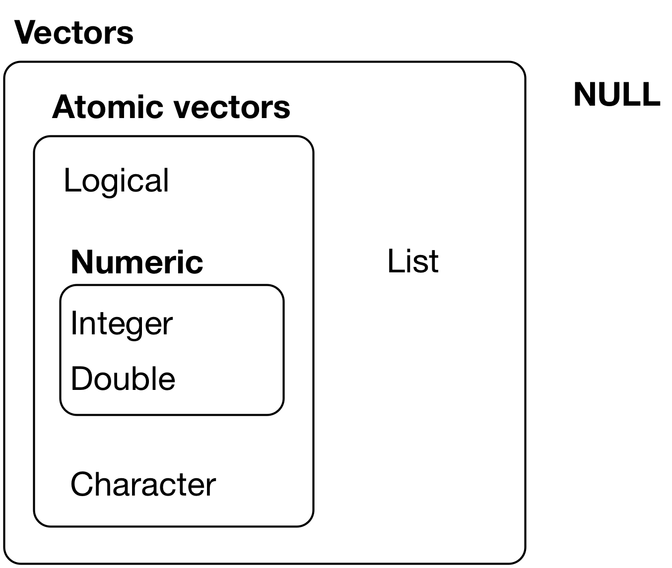
Credit: R for Data Science

Basic data types:

Logical (TRUE, FALSE)
Numeric (e.g., 5, 2.5)
Integer (e.g., 1L, 4L, where L tells R to store as integer type)
Character (e.g., "R is fun")

Basic data structures:

Atomic vectors
Lists
- Dataframes

2.1 Atomtic vectors

What are atomic vectors?

Atomic vectors are objects that contains elements
Elements must be of the same data type (i.e., homogeneous)
The class() and typeof() a vector describes the elements it contains

Example: Investigating logical vectors

v <- c(TRUE, FALSE, FALSE, TRUE)
str(v)
#>  logi [1:4] TRUE FALSE FALSE TRUE
class(v)
#> [1] "logical"
typeof(v)
#> [1] "logical"

Example: Investigating numeric vectors

v <- c(1, 3, 5, 7)
str(v)
#>  num [1:4] 1 3 5 7
class(v)
#> [1] "numeric"
typeof(v)
#> [1] "double"

Example: Investigating integer vectors

v <- c(1L, 3L, 5L, 7L)
str(v)
#>  int [1:4] 1 3 5 7
class(v)
#> [1] "integer"
typeof(v)
#> [1] "integer"

Example: Investigating character vectors

Each element in a character vector is a string (covered in next section):

v <- c("a", "b", "c", "d")
str(v)
#>  chr [1:4] "a" "b" "c" "d"
class(v)
#> [1] "character"
typeof(v)
#> [1] "character"

2.2 Lists

What are lists?

Lists are objects that contains elements
Elements do not need to be of the same type (i.e., heterogeneous)
- Elements can be atomic vectors or even other lists
The class() and typeof() a list is list

Example: Investigating heterogeneous lists

l <- list(2.5, "abc", TRUE, c(1L, 2L, 3L))
str(l)
#> List of 4
#>  $ : num 2.5
#>  $ : chr "abc"
#>  $ : logi TRUE
#>  $ : int [1:3] 1 2 3
class(l)
#> [1] "list"
typeof(l)
#> [1] "list"

Example: Investigating nested lists

l <- list(list(TRUE, c(1, 2, 3), list(c("a", "b", "c"))), FALSE, 10L)
str(l)
#> List of 3
#>  $ :List of 3
#>   ..$ : logi TRUE
#>   ..$ : num [1:3] 1 2 3
#>   ..$ :List of 1
#>   .. ..$ : chr [1:3] "a" "b" "c"
#>  $ : logi FALSE
#>  $ : int 10
class(l)
#> [1] "list"
typeof(l)
#> [1] "list"

2.2.1 Dataframes

What are dataframes?

Dataframes are a special kind of list with the following characteristics:
- Each element is a vector (i.e., a column in the dataframe)
- The element should be named (i.e., column name in the dataframe)
- Each of the vectors must be the same length (i.e., same number of rows in the dataframe)
- The data type of each vector may be different
Dataframes can be created using the function data.frame()
The class() of a dataframe is data.frame
The typeof() a dataframe is list

Example: Investigating dataframe

df <- data.frame(
  colA = c(1, 2, 3),
  colB = c("a", "b", "c"),
  colC = c(TRUE, FALSE, TRUE),
  stringsAsFactors = FALSE
)
df
#> # A tibble: 3 × 3
#>    colA colB  colC 
#>   <dbl> <chr> <lgl>
#> 1     1 a     TRUE 
#> 2     2 b     FALSE
#> 3     3 c     TRUE
str(df)
#> 'data.frame':    3 obs. of  3 variables:
#>  $ colA: num  1 2 3
#>  $ colB: chr  "a" "b" "c"
#>  $ colC: logi  TRUE FALSE TRUE
class(df)
#> [1] "data.frame"
typeof(df)
#> [1] "list"

2.3 Converting between types

Functions for converting between types:

as.logical(): Convert to logical
as.numeric(): Convert to numeric
as.integer(): Convert to integer
as.character(): Convert to character
as.list(): Convert to list
as.data.frame(): Convert to data.frame

Example: Using as.logical() to convert to logical

Character vector coerced to logical vector:

# Only "TRUE"/"FALSE", "True"/"False", "T"/"F", "true"/"false" are able to be coerced to logical type
as.logical(c("TRUE", "FALSE", "True", "False", "true", "false", "T", "F", "t", "f", ""))
#>  [1]  TRUE FALSE  TRUE FALSE  TRUE FALSE  TRUE FALSE    NA    NA    NA

Numeric vector coerced to logical vector:

# 0 is treated as FALSE, while all other numeric values are treated as TRUE
as.logical(c(0, 0.0, 1, -1, 20, 5.5))
#> [1] FALSE FALSE  TRUE  TRUE  TRUE  TRUE

Example: Using as.numeric() to convert to numeric

Logical vector coerced to numeric vector:

# FALSE is mapped to 0 and TRUE is mapped to 1
as.numeric(c(FALSE, TRUE))
#> [1] 0 1

Character vector coerced to numeric vector:

# Strings containing numeric values can be coerced to numeric (leading 0's are dropped) 
# All other characters become NA
as.numeric(c("0", "007", "2.5", "abc", "."))
#> [1] 0.0 7.0 2.5  NA  NA

Example: Using as.integer() to convert to integer

Logical vector coerced to integer vector:

# FALSE is mapped to 0 and TRUE is mapped to 1
as.integer(c(FALSE, TRUE))
#> [1] 0 1

Character vector coerced to integer vector:

# Strings containing numeric values can be coerced to integer (leading 0's are dropped, decimals are truncated) 
# All other characters become NA
as.integer(c("0", "007", "2.5", "abc", "."))
#> [1]  0  7  2 NA NA

Numeric vector coerced to integer vector:

# All decimal places are truncated
as.integer(c(0, 2.1, 10.5, 8.8, -1.8))
#> [1]  0  2 10  8 -1

Example: Using as.character() to convert to character

Logical vector coerced to character vector:

as.character(c(FALSE, TRUE))
#> [1] "FALSE" "TRUE"

Numeric vector coerced to character vector:

as.character(c(-5, 0, 2.5))
#> [1] "-5"  "0"   "2.5"

Integer vector coerced to character vector:

as.character(c(-2L, 0L, 10L))
#> [1] "-2" "0"  "10"

Example: Using as.list() to convert to list

Atomic vectors coerced to list:

# Logical vector
as.list(c(TRUE, FALSE))
#> [[1]]
#> [1] TRUE
#> 
#> [[2]]
#> [1] FALSE

# Character vector
as.list(c("a", "b", "c"))
#> [[1]]
#> [1] "a"
#> 
#> [[2]]
#> [1] "b"
#> 
#> [[3]]
#> [1] "c"

# Numeric vector
as.list(1:3)
#> [[1]]
#> [1] 1
#> 
#> [[2]]
#> [1] 2
#> 
#> [[3]]
#> [1] 3

Example: Using as.data.frame() to convert to data.frame

Lists coerced to dataframe:

# Create a list
l <- list(A = c("x", "y", "z"), B = c(1, 2, 3))
str(l)
#> List of 2
#>  $ A: chr [1:3] "x" "y" "z"
#>  $ B: num [1:3] 1 2 3

# Convert to class `data.frame`
df <- as.data.frame(l, stringsAsFactors = F)
str(df)
#> 'data.frame':    3 obs. of  2 variables:
#>  $ A: chr  "x" "y" "z"
#>  $ B: num  1 2 3

Example: Practical example of converting type

When working with data, it may be helpful to label values for certain variables. Data files often come with a codebook that defines how values are coded. Let’s look at an example of labeling values and how converting data type may come into play.

We’ll look at the FIPS variable from the Integrated Postsecondary Education Data System (IPEDS) data. The state FIPS code is a numeric code that identifies a state. For example, 1 is the FIPS code for Alabama, 2 is the FIPS code for Alaska, etc. We’ll want to label each numeric value in the FIPS column with the corresponding state name.

# Library for labeling variables and values in a dataframe
library(labelled)

# Read in IPEDS data and codebook
ipeds_df <- read.csv('https://raw.githubusercontent.com/cyouh95/recruiting-chapter/master/data/ipeds_hd2017.csv', header = TRUE, na.strings=c('', 'NA'), stringsAsFactors = F)
ipeds_values <- read.csv('https://raw.githubusercontent.com/cyouh95/recruiting-chapter/master/data/ipeds_hd2017_values.csv', header = TRUE, na.strings=c('', 'NA'), stringsAsFactors = F)

# The codebook defines how variables are coded, such as STABBR, FIPS, and other variables
head(ipeds_values)
#> # A tibble: 6 × 6
#>   varnumber varname codevalue valuelabel frequency percent
#>       <int> <chr>   <chr>     <chr>          <int>   <dbl>
#> 1     10016 STABBR  AL        Alabama           95    1.33
#> 2     10016 STABBR  AK        Alaska            10    0.14
#> 3     10016 STABBR  AZ        Arizona          137    1.92
#> 4     10016 STABBR  AR        Arkansas          86    1.2 
#> 5     10016 STABBR  CA        California       729   10.2 
#> 6     10016 STABBR  CO        Colorado         118    1.65

# Filter codebook for just the values for the FIPS variable
fips_values <- ipeds_values %>% filter(varname == 'FIPS') %>% select(varname, codevalue, valuelabel)
head(fips_values)
#> # A tibble: 6 × 3
#>   varname codevalue valuelabel
#>   <chr>   <chr>     <chr>     
#> 1 FIPS    1         Alabama   
#> 2 FIPS    2         Alaska    
#> 3 FIPS    4         Arizona   
#> 4 FIPS    5         Arkansas  
#> 5 FIPS    6         California
#> 6 FIPS    8         Colorado

When we read in the data from the CSV files, R automatically tries to determine the data type of each variable. As seen below, the FIPS column from the ipeds_df that we want to label is of type integer, while the codevalue column from the codebook is of type character (since not all values are numeric):

# Type of `FIPS` column
str(ipeds_df$FIPS)
#>  int [1:7153] 1 1 1 1 1 1 1 1 1 1 ...

# Type of `codevalue` column
str(fips_values$codevalue)
#>  chr [1:59] "1" "2" "4" "5" "6" "8" "9" "10" "11" "12" "13" "15" "16" "17" ...

This discrepancy becomes a problem when we try to label the value using the labelled library:

# Error: `x` and `labels` must be same type
val_label(ipeds_df$FIPS, fips_values[1, 'codevalue']) <- fips_values[1, 'valuelabel']

To resolve this, we can use as.integer() to convert the codevalue from character type to integer before trying to label the value:

# This now works
val_label(ipeds_df$FIPS, as.integer(fips_values[1, 'codevalue'])) <- fips_values[1, 'valuelabel']

# Check value labels
val_labels(ipeds_df$FIPS)
#> Alabama 
#>       1

# We can use as.integer() to convert the entire vector (ie. codevalue column) to integer
fips_values$codevalue <- as.integer(fips_values$codevalue)

# Type of `codevalue` column
str(fips_values$codevalue)
#>  int [1:59] 1 2 4 5 6 8 9 10 11 12 ...

# Use loop to label the rest of the values
for (i in 1:nrow(fips_values)) {
  val_label(ipeds_df$FIPS, fips_values[i, 'codevalue']) <- fips_values[i, 'valuelabel']
}

# Check value labels
val_labels(ipeds_df$FIPS)
#>                        Alabama                         Alaska 
#>                              1                              2 
#>                        Arizona                       Arkansas 
#>                              4                              5 
#>                     California                       Colorado 
#>                              6                              8 
#>                    Connecticut                       Delaware 
#>                              9                             10 
#>           District of Columbia                        Florida 
#>                             11                             12 
#>                        Georgia                         Hawaii 
#>                             13                             15 
#>                          Idaho                       Illinois 
#>                             16                             17 
#>                        Indiana                           Iowa 
#>                             18                             19 
#>                         Kansas                       Kentucky 
#>                             20                             21 
#>                      Louisiana                          Maine 
#>                             22                             23 
#>                       Maryland                  Massachusetts 
#>                             24                             25 
#>                       Michigan                      Minnesota 
#>                             26                             27 
#>                    Mississippi                       Missouri 
#>                             28                             29 
#>                        Montana                       Nebraska 
#>                             30                             31 
#>                         Nevada                  New Hampshire 
#>                             32                             33 
#>                     New Jersey                     New Mexico 
#>                             34                             35 
#>                       New York                 North Carolina 
#>                             36                             37 
#>                   North Dakota                           Ohio 
#>                             38                             39 
#>                       Oklahoma                         Oregon 
#>                             40                             41 
#>                   Pennsylvania                   Rhode Island 
#>                             42                             44 
#>                 South Carolina                   South Dakota 
#>                             45                             46 
#>                      Tennessee                          Texas 
#>                             47                             48 
#>                           Utah                        Vermont 
#>                             49                             50 
#>                       Virginia                     Washington 
#>                             51                             53 
#>                  West Virginia                      Wisconsin 
#>                             54                             55 
#>                        Wyoming                 American Samoa 
#>                             56                             60 
#> Federated States of Micronesia                           Guam 
#>                             64                             66 
#>               Marshall Islands              Northern Marianas 
#>                             68                             69 
#>                          Palau                    Puerto Rico 
#>                             70                             72 
#>                 Virgin Islands 
#>                             78

3 String basics

What are strings?

String is a type of data in R
You can create strings using either single quotes (') or double quotes (")
- Internally, R stores strings using double quotes
The class() and typeof() a string is character

Example: Creating string using single quotes

Notice how R stores strings using double quotes internally:

my_string <- 'This is a string'
my_string
#> [1] "This is a string"

Example: Creating string using double quotes

my_string <- "Strings can also contain numbers: 123"
my_string
#> [1] "Strings can also contain numbers: 123"

Example: Checking class and type of strings

class(my_string)
#> [1] "character"
typeof(my_string)
#> [1] "character"

Note: To include quotes as part of the string, we can either use the other type of quotes to surround the string (i.e., ' or ") or escape the quote using a backslash (\). We won’t be going in-depth into escaping characters for this class, but see appendix for more details if you are interested.

# Include quote by using the other type of quotes to surround the string 
my_string <- "There's no issues with this string."
my_string
#> [1] "There's no issues with this string."

# Include quote of the same type by escaping it with a backslash
my_string <- 'There\'s no issues with this string.'
my_string
#> [1] "There's no issues with this string."

# This would not work
my_string <- 'There's an issue with this string.'
my_string

4 `stringr` package

“A consistent, simple and easy to use set of wrappers around the fantastic stringi package. All function and argument names (and positions) are consistent, all functions deal with NA’s and zero length vectors in the same way, and the output from one function is easy to feed into the input of another.”

Credit: stringr R documentation

The stringr package:

The stringr package is based off the stringi package and is part of Tidyverse
stringr contains functions to work with strings
For many functions in the stringr package, there are equivalent “base R” functions
But stringr functions all follow the same rules, while rules often differ across different “base R” string functions, so we will focus exclusively on stringr functions
Most stringr functions start with str_ (e.g., str_length)

4.1 `str_length()`

The str_length() function:

?str_length

# SYNTAX
str_length(string)

Function: Find string length
Arguments:
- string: Character vector (or vector coercible to character)
Note that str_length() calculates the length of a string, whereas the length() function (which is not part of stringr package) calculates the number of elements in an object

Example: Using str_length() on string

str_length("cats")
#> [1] 4

Compare to length(), which treats the string as a single object:

length("cats")
#> [1] 1

Example: Using str_length() on character vector

str_length(c("cats", "in", "hat"))
#> [1] 4 2 3

Compare to length(), which finds the number of elements in the vector:

length(c("cats", "in", "hat"))
#> [1] 3

Example: Using str_length() on other vectors coercible to character

Logical vectors can be coerced to character vectors:

str_length(c(TRUE, FALSE))
#> [1] 4 5

Numeric vectors can be coerced to character vectors:

str_length(c(1, 2.5, 3000))
#> [1] 1 3 4

Integer vectors can be coerced to character vectors:

str_length(c(2L, 100L))
#> [1] 1 3

Example: Using str_length() on dataframe column

Recall that the columns in a dataframe are just vectors, so we can use str_length() as long as the vector is coercible to character type. Let’s look at the screen_name column from the p12_df:

# `p12_df` is a dataframe object
str(p12_df)
#> tibble [328 × 5] (S3: tbl_df/tbl/data.frame)
#>  $ user_id    : chr [1:328] "22080148" "22080148" "22080148" "22080148" ...
#>  $ created_at : POSIXct[1:328], format: "2020-04-25 22:37:18" "2020-04-23 21:11:49" ...
#>  $ screen_name: chr [1:328] "WSUPullman" "WSUPullman" "WSUPullman" "WSUPullman" ...
#>  $ text       : chr [1:328] "Big Dez is headed to Indy!\n\n#GoCougs | #NFLDraft2020 | @dadpat7 | @Colts | #NFLCougs https://t.co/NdGsvXnij7" "Cougar Cheese. That's it. That's the tweet. 🧀#WSU #GoCougs https://t.co/0OWGvQlRZs" "Darien McLaughlin '19, and her dog, Yuki, went on a #Pullman distance walk this weekend. We will let you judge "| __truncated__ "6 houses, one pick. Cougs, which one you got? Reply ⬇️  #WSU #CougsContain #GoCougs https://t.co/lNDx7r71b2" ...
#>  $ location   : chr [1:328] "Pullman, Washington USA" "Pullman, Washington USA" "Pullman, Washington USA" "Pullman, Washington USA" ...

# `screen_name` column is a character vector
str(p12_df$screen_name)
#>  chr [1:328] "WSUPullman" "WSUPullman" "WSUPullman" "WSUPullman" ...

[Base R method] Use str_length() to calculate the length of each screen_name:

# Let's focus on just the unique screen names
unique(p12_df$screen_name)
#>  [1] "WSUPullman"      "CalAdmissions"   "UW"              "USCAdmission"   
#>  [5] "uoregon"         "FutureSunDevils" "UCLAAdmission"   "UtahAdmissions" 
#>  [9] "futurebuffs"     "uaadmissions"    "BeaverVIP"

str_length(unique(p12_df$screen_name))
#>  [1] 10 13  2 12  7 15 13 14 11 12  9

[Tidyverse method] Use str_length() to calculate the length of each screen_name:

# Let's focus on just the unique screen names
p12_df %>% select(screen_name) %>% unique()
#> # A tibble: 11 × 1
#>    screen_name    
#>    <chr>          
#>  1 WSUPullman     
#>  2 CalAdmissions  
#>  3 UW             
#>  4 USCAdmission   
#>  5 uoregon        
#>  6 FutureSunDevils
#>  7 UCLAAdmission  
#>  8 UtahAdmissions 
#>  9 futurebuffs    
#> 10 uaadmissions   
#> 11 BeaverVIP

#p12_df %>% select(screen_name) %>% unique() %>% str_length()

Notice that the above line does not work as expected because we passed in a dataframe to str_length() and it is trying to coerce that to character:

class(p12_df %>% select(screen_name) %>% unique())
#> [1] "tbl_df"     "tbl"        "data.frame"

An alternative way is to add a column to the dataframe that contains the result of applying str_length() to the screen_name vector:

p12_df %>% select(screen_name) %>% unique() %>% 
  mutate(screen_name_len = str_length(screen_name))
#> # A tibble: 11 × 2
#>    screen_name     screen_name_len
#>    <chr>                     <int>
#>  1 WSUPullman                   10
#>  2 CalAdmissions                13
#>  3 UW                            2
#>  4 USCAdmission                 12
#>  5 uoregon                       7
#>  6 FutureSunDevils              15
#>  7 UCLAAdmission                13
#>  8 UtahAdmissions               14
#>  9 futurebuffs                  11
#> 10 uaadmissions                 12
#> 11 BeaverVIP                     9

4.2 `str_c()`

The str_c() function:

?str_c

# SYNTAX AND DEFAULT VALUES
str_c(..., sep = "", collapse = NULL)

Function: Concatenate strings between vectors (element-wise)
Arguments:
- The input is one or more character vectors (or vectors coercible to character)
  - Zero length arguments are removed
  - Short arguments are recycled to the length of the longest
- sep: String to insert between input vectors
- collapse: Optional string used to combine input vectors into single string

Example: Using str_c() on one vector

Since we only provided one input vector, it has nothing to concatenate with, so str_c() will just return the same vector:

str_c(c("a", "b", "c"))
#> [1] "a" "b" "c"

Note that specifying the sep argument will also not have any effect because we only have one input vector, and sep is the separator between multiple vectors:

str_c(c("a", "b", "c"), sep = "~")
#> [1] "a" "b" "c"

# Check length: Output is the original vector of 3 elements
str_c(c("a", "b", "c")) %>% length()
#> [1] 3

As seen above, str_c() returns a vector by default (because the default value for the collapse argument is NULL). But we can specify a string for collapse in order to collapse the elements of the output vector into a single string:

str_c(c("a", "b", "c"), collapse = "|")
#> [1] "a|b|c"

# Check length: Output vector of length 3 is collapsed into a single string
str_c(c("a", "b", "c"), collapse = "|") %>% length()
#> [1] 1

# Check str_length: This gives the length of the collapsed string, which is 5 characters long
str_c(c("a", "b", "c"), collapse = "|") %>% str_length()
#> [1] 5

Example: Using str_c() on more than one vector

When we provide multiple input vectors, we can see that the vectors get concatenated element-wise (i.e., 1st element from each vector are concatenated, 2nd element from each vector are concatenated, etc):

str_c(c("a", "b", "c"), c("x", "y", "z"), c("!", "?", ";"))
#> [1] "ax!" "by?" "cz;"

The default separator for each element-wise concatenation is an empty string (""), but we can customize that by specifying the sep argument:

str_c(c("a", "b", "c"), c("x", "y", "z"), c("!", "?", ";"), sep = "~")
#> [1] "a~x~!" "b~y~?" "c~z~;"

# Check length: Output vector is same length as input vectors
str_c(c("a", "b", "c"), c("x", "y", "z"), c("!", "?", ";"), sep = "~") %>% length()
#> [1] 3

Again, we can specify the collapse argument in order to collapse the elements of the output vector into a single string:

str_c(c("a", "b", "c"), c("x", "y", "z"), c("!", "?", ";"), collapse = "|")
#> [1] "ax!|by?|cz;"

# Check length: Output vector of length 3 is collapsed into a single string
str_c(c("a", "b", "c"), c("x", "y", "z"), c("!", "?", ";"), collapse = "|") %>% length()
#> [1] 1

# Specifying both `sep` and `collapse`
str_c(c("a", "b", "c"), c("x", "y", "z"), c("!", "?", ";"), sep = "~", collapse = "|")
#> [1] "a~x~!|b~y~?|c~z~;"

Example: Using str_c() on “strings”

What do we mean by “strings”?

Informally, We can think of a “string” as being a character vector with length() equal to 1 (i.e., one element).
Another way to think of it, a “string” is anything you put in between quotes”.
Loosely, we can also think of individual elements within a character vector as strings

Below, passing 3 strings into str_c() is like passing in 3 vectors of size 1 each.

Remember that vectors are concatenated element-wise, so these strings will be joined like this:

str_c("a", "b", "c")
#> [1] "abc"

# Again, we can think of strings as being character vectors of size 1
str_c(c("a"), c("b"), c("c"))
#> [1] "abc"

We can use sep to specify how the elements are separated:

str_c("a", "b", "c", sep = "~")
#> [1] "a~b~c"

Since we only have 1 element in each vector, the output from str_c() is a vector of length 1. Thus, collapse will not be useful here since it works to collapse multiple elements in the output vector into a single string:

str_c("a", "b", "c", collapse = "|")
#> [1] "abc"

Example: Using str_c() on types other than character

When we provide a non-character vector (such as a numeric or logical vector), it will get coerced into a character vector:

str_c(c("a", "b", "c"), c(1, 2, 3), c(TRUE, FALSE, FALSE))
#> [1] "a1TRUE"  "b2FALSE" "c3FALSE"

# Specifying both `sep` and `collapse`
str_c(c("a", "b", "c"), c(1, 2, 3), c(TRUE, FALSE, FALSE), sep = "~", collapse = "|")
#> [1] "a~1~TRUE|b~2~FALSE|c~3~FALSE"

Note that we can also use any other single element input (other than string) that can be coerced to character:

str_c(TRUE, 1.5, 2L, "X")
#> [1] "TRUE1.52X"

Example: Using str_c() on vectors of different lengths

When multiple vectors are provided, they are joined together element-wise, recycling the elements of the shorter vectors:

str_c("#", c("a", "b", "c", "d"), c(1, 2, 3), c(TRUE, FALSE))
#> [1] "#a1TRUE"  "#b2FALSE" "#c3TRUE"  "#d1FALSE"

# Specifying both `sep` and `collapse`
str_c("#", c("a", "b", "c", "d"), c(1, 2, 3), c(TRUE, FALSE), sep = "~", collapse = "|")
#> [1] "#~a~1~TRUE|#~b~2~FALSE|#~c~3~TRUE|#~d~1~FALSE"

Example: Using str_c() on dataframe columns

Let’s combine the user_id and screen_name columns from p12_df. We’ll focus on unique Twitter handles:

p12_unique_df <- p12_df %>% select(user_id, screen_name) %>% unique()
p12_unique_df
#> # A tibble: 11 × 2
#>    user_id    screen_name    
#>    <chr>      <chr>          
#>  1 22080148   WSUPullman     
#>  2 15988549   CalAdmissions  
#>  3 27103822   UW             
#>  4 198643896  USCAdmission   
#>  5 40940457   uoregon        
#>  6 325014504  FutureSunDevils
#>  7 2938776590 UCLAAdmission  
#>  8 4922145709 UtahAdmissions 
#>  9 45879674   futurebuffs    
#> 10 44733626   uaadmissions   
#> 11 403743606  BeaverVIP

[Base R method] Use str_c() to combine user_id and screen_name:

str_c(p12_unique_df$user_id, "=", p12_unique_df$screen_name, sep = " ", collapse = ", ")
#> [1] "22080148 = WSUPullman, 15988549 = CalAdmissions, 27103822 = UW, 198643896 = USCAdmission, 40940457 = uoregon, 325014504 = FutureSunDevils, 2938776590 = UCLAAdmission, 4922145709 = UtahAdmissions, 45879674 = futurebuffs, 44733626 = uaadmissions, 403743606 = BeaverVIP"
str_c(p12_unique_df$user_id, "=", p12_unique_df$screen_name, sep = " ") # without collapsing to one element
#>  [1] "22080148 = WSUPullman"       "15988549 = CalAdmissions"   
#>  [3] "27103822 = UW"               "198643896 = USCAdmission"   
#>  [5] "40940457 = uoregon"          "325014504 = FutureSunDevils"
#>  [7] "2938776590 = UCLAAdmission"  "4922145709 = UtahAdmissions"
#>  [9] "45879674 = futurebuffs"      "44733626 = uaadmissions"    
#> [11] "403743606 = BeaverVIP"

[Tidyverse method] Use str_c() to combine user_id and screen_name:

p12_unique_df %>% mutate(twitter_handle = str_c(user_id,screen_name))
#> # A tibble: 11 × 3
#>    user_id    screen_name     twitter_handle          
#>    <chr>      <chr>           <chr>                   
#>  1 22080148   WSUPullman      22080148WSUPullman      
#>  2 15988549   CalAdmissions   15988549CalAdmissions   
#>  3 27103822   UW              27103822UW              
#>  4 198643896  USCAdmission    198643896USCAdmission   
#>  5 40940457   uoregon         40940457uoregon         
#>  6 325014504  FutureSunDevils 325014504FutureSunDevils
#>  7 2938776590 UCLAAdmission   2938776590UCLAAdmission 
#>  8 4922145709 UtahAdmissions  4922145709UtahAdmissions
#>  9 45879674   futurebuffs     45879674futurebuffs     
#> 10 44733626   uaadmissions    44733626uaadmissions    
#> 11 403743606  BeaverVIP       403743606BeaverVIP

p12_unique_df %>% mutate(twitter_handle = str_c("User #", user_id, " is @", screen_name))
#> # A tibble: 11 × 3
#>    user_id    screen_name     twitter_handle                     
#>    <chr>      <chr>           <chr>                              
#>  1 22080148   WSUPullman      User #22080148 is @WSUPullman      
#>  2 15988549   CalAdmissions   User #15988549 is @CalAdmissions   
#>  3 27103822   UW              User #27103822 is @UW              
#>  4 198643896  USCAdmission    User #198643896 is @USCAdmission   
#>  5 40940457   uoregon         User #40940457 is @uoregon         
#>  6 325014504  FutureSunDevils User #325014504 is @FutureSunDevils
#>  7 2938776590 UCLAAdmission   User #2938776590 is @UCLAAdmission 
#>  8 4922145709 UtahAdmissions  User #4922145709 is @UtahAdmissions
#>  9 45879674   futurebuffs     User #45879674 is @futurebuffs     
#> 10 44733626   uaadmissions    User #44733626 is @uaadmissions    
#> 11 403743606  BeaverVIP       User #403743606 is @BeaverVIP

4.3 `str_sub()`

The str_sub() function:

?str_sub

# SYNTAX AND DEFAULT VALUES
str_sub(string, start = 1L, end = -1L)
str_sub(string, start = 1L, end = -1L, omit_na = FALSE) <- value

Function: Subset strings
Arguments:
- string: Character vector (or vector coercible to character)
- start: Position of first character to be included in substring (default: 1)
- end: Position of last character to be included in substring (default: -1)
  - Negative index means counting backwards from the end of the string
  - If an element in the vector is shorter than the specified end, it will just include all the available characters that it does have
- omit_na: If TRUE, missing values in any of the arguments provided will result in an unchanged input
When str_sub() is used in the assignment form, you can replace the subsetted part of the string with a value of your choice
- If an element in the vector is too short to meet the subset specification, the replacement value will be concatenated to the end of that element
- Note that this modifies your input vector directly, so you must have the vector saved to a variable (see example below)

Example: Using str_sub() to subset strings

If no start and end positions are specified, str_sub() will by default return the entire (original) string:

str_sub(string = c("abcdefg", 123, TRUE))
#> [1] "abcdefg" "123"     "TRUE"

Note that if an element is shorter than the specified end (i.e., 123 in the example below), it will just include all the available characters that it does have:

str_sub(string = c("abcdefg", 123, TRUE), start = 2, end = 4)
#> [1] "bcd" "23"  "RUE"

Remember we can also use negative index to count the position starting from the back:

str_sub(c("abcdefg", 123, TRUE), start = 2, end = -2)
#> [1] "bcdef" "2"     "RU"

Example: Using str_sub() to replace strings

If no start and end positions are specified, str_sub() will by default return the original string, so the entire string would be replaced:

v <- c("A", "AB", "ABC", "ABCD", "ABCDE")
str_sub(v, start = 1,end =-1)
#> [1] "A"     "AB"    "ABC"   "ABCD"  "ABCDE"

str_sub(v, start = 1,end =-1) <- "*"
v
#> [1] "*" "*" "*" "*" "*"

If an element in the vector is too short to meet the subset specification, the replacement value will be concatenated to the end of that element:

v <- c("A", "AB", "ABC", "ABCD", "ABCDE")
v
#> [1] "A"     "AB"    "ABC"   "ABCD"  "ABCDE"
str_sub(v, start = 2, end = 3)
#> [1] ""   "B"  "BC" "BC" "BC"

str_sub(v, start = 2, end = 3) <- "*"
v
#> [1] "A*"   "A*"   "A*"   "A*D"  "A*DE"

Note that because the replacement form of str_sub() modifies the input vector directly, we need to save it in a variable first. Directly passing in the vector to str_sub() would give us an error:

# Does not work
str_sub(c("A", "AB", "ABC", "ABCD", "ABCDE")) <- "*"

Example: Using str_sub() on dataframe column

We can use as.character() to turn the created_at value to a string, then use str_sub() to extract out various date/time components from the string:

p12_datetime_df <- p12_df %>% select(created_at) %>%
  mutate(
      dt_chr = as.character(created_at),
      date_chr = str_sub(dt_chr, 1, 10),
      yr_chr = str_sub(dt_chr, 1, 4),
      mth_chr = str_sub(dt_chr, 6, 7),
      day_chr = str_sub(dt_chr, 9, 10),
      hr_chr = str_sub(dt_chr, -8, -7),
      min_chr = str_sub(dt_chr, -5, -4),
      sec_chr = str_sub(dt_chr, -2, -1)
    )
p12_datetime_df
#> # A tibble: 328 × 9
#>    created_at          dt_chr      date_…¹ yr_chr mth_chr day_chr hr_chr min_chr
#>    <dttm>              <chr>       <chr>   <chr>  <chr>   <chr>   <chr>  <chr>  
#>  1 2020-04-25 22:37:18 2020-04-25… 2020-0… 2020   04      25      22     37     
#>  2 2020-04-23 21:11:49 2020-04-23… 2020-0… 2020   04      23      21     11     
#>  3 2020-04-21 04:00:00 2020-04-21… 2020-0… 2020   04      21      04     00     
#>  4 2020-04-24 03:00:00 2020-04-24… 2020-0… 2020   04      24      03     00     
#>  5 2020-04-20 19:00:21 2020-04-20… 2020-0… 2020   04      20      19     00     
#>  6 2020-04-20 02:20:01 2020-04-20… 2020-0… 2020   04      20      02     20     
#>  7 2020-04-22 04:00:00 2020-04-22… 2020-0… 2020   04      22      04     00     
#>  8 2020-04-25 17:00:00 2020-04-25… 2020-0… 2020   04      25      17     00     
#>  9 2020-04-21 15:13:06 2020-04-21… 2020-0… 2020   04      21      15     13     
#> 10 2020-04-21 17:52:47 2020-04-21… 2020-0… 2020   04      21      17     52     
#> # … with 318 more rows, 1 more variable: sec_chr <chr>, and abbreviated
#> #   variable name ¹date_chr

4.4 Other `stringr` functions

Other useful stringr functions:

str_to_upper(): Turn strings to uppercase
str_to_lower(): Turn strings to lowercase
str_sort(): Sort a character vector
str_trim(): Trim whitespace from strings (including \n, \t, etc.)
str_pad(): Pad strings with specified character

Example: Using str_to_upper() to turn strings to uppercase

Turn column names of p12_df to uppercase:

# Column names are originally lowercase
names(p12_df)
#> [1] "user_id"     "created_at"  "screen_name" "text"        "location"

# Turn column names to uppercase
names(p12_df) <- str_to_upper(names(p12_df))
names(p12_df)
#> [1] "USER_ID"     "CREATED_AT"  "SCREEN_NAME" "TEXT"        "LOCATION"

Example: Using str_to_lower() to turn strings to lowercase

Turn column names of p12_df to lowercase:

# Column names are originally uppercase
names(p12_df)
#> [1] "USER_ID"     "CREATED_AT"  "SCREEN_NAME" "TEXT"        "LOCATION"

# Turn column names to lowercase
names(p12_df) <- str_to_lower(names(p12_df))
names(p12_df)
#> [1] "user_id"     "created_at"  "screen_name" "text"        "location"

Example: Using str_sort() to sort character vector

Sort the vector of p12_df column names:

# Before sort
names(p12_df)
#> [1] "user_id"     "created_at"  "screen_name" "text"        "location"

# Sort alphabetically (default)
str_sort(names(p12_df))
#> [1] "created_at"  "location"    "screen_name" "text"        "user_id"

# Sort reverse alphabetically
str_sort(names(p12_df), decreasing = TRUE)
#> [1] "user_id"     "text"        "screen_name" "location"    "created_at"

Example: Using str_trim() to trim whitespace from string

# Trim whitespace from both left and right sides (default)
str_trim(c("\nABC ", " XYZ\t"))
#> [1] "ABC" "XYZ"

# Trim whitespace from left side
str_trim(c("\nABC ", " XYZ\t"), side = "left")
#> [1] "ABC "  "XYZ\t"

# Trim whitespace from right side
str_trim(c("\nABC ", " XYZ\t"), side = "right")
#> [1] "\nABC" " XYZ"

Example: Using str_pad() to pad string with character

Let’s say we have a vector of zip codes that has lost all leading 0’s. We can use str_pad() to add that back in:

# Pad the left side of strings with "0" until width of 5 is reached
str_pad(c(95035, 90024, 5009, 5030), width = 5, side = "left", pad = "0")
#> [1] "95035" "90024" "05009" "05030"

5 Dates and times

“Date-time data can be frustrating to work with in R. R commands for date-times are generally unintuitive and change depending on the type of date-time object being used. Moreover, the methods we use with date-times must be robust to time zones, leap days, daylight savings times, and other time related quirks, and R lacks these capabilities in some situations. Lubridate makes it easier to do the things R does with date-times and possible to do the things R does not.”

Credit: lubridate documentation

How are dates and times stored in R? (From Dates and Times in R)

The Date class is used for storing dates
- “Internally, Date objects are stored as the number of days since January 1, 1970, using negative numbers for earlier dates. The as.numeric() function can be used to convert a Date object to its internal form.”
POSIX classes can be used for storing date plus times
- “The POSIXct class stores date/time values as the number of seconds since January 1, 1970”
- “The POSIXlt class stores date/time values as a list of components (hour, min, sec, mon, etc.) making it easy to extract these parts”
There is no native R class for storing only time

Why use date/time objects?

Using date/time objects makes it easier to fetch or modify various date/time components (e.g., year, month, day, day of the week)
- Compared to if the date/time is just stored in a string, these components are not as readily accessible and need to be parsed
You can perform certain arithmetics with date/time objects (e.g., find the “difference” between date/time points)

5.1 Creating date/time objects

5.1.1 Creating date/time objects by parsing input

Functions that create date/time objects by parsing character or numeric input:

Create Date object: ymd(), ydm(), mdy(), myd(), dmy(), dym()
- y stands for year, m stands for month, d stands for day
- Select the function that represents the order in which your date input is formatted, and the function will be able to parse your input and create a Date object
Create POSIXct object: ymd_h(), ymd_hm(), ymd_hms(), etc.
- h stands for hour, m stands for minute, s stands for second
- For any of the previous 6 date functions, you can append h, hm, or hms if you want to provide additional time information in order to create a POSIXct object
- To force a POSIXct object without providing any time information, you can just provide a timezone (using tz) to one of the date functions and it will assume midnight as the time
- You can use Sys.timezone() to get the timezone for your location

Example: Creating Date object from character or numeric input

The lubridate functions are flexible and can parse dates in various formats:

d <- mdy("1/1/2020")
d
#> [1] "2020-01-01"

d <- mdy("1-1-2020")
d
#> [1] "2020-01-01"

d <- mdy("Jan. 1, 2020")
d
#> [1] "2020-01-01"

d <- ymd(20200101)
d
#> [1] "2020-01-01"

Investigate the Date object:

class(d)
#> [1] "Date"
typeof(d)
#> [1] "double"

# Number of days since January 1, 1970
as.numeric(d)
#> [1] 18262

Example: Creating POSIXct object from character or numeric input

The lubridate functions are flexible and can parse AM/PM in various formats:

dt <- mdy_h("12/31/2019 11pm")
dt
#> [1] "2019-12-31 23:00:00 UTC"

dt <- mdy_hm("12/31/2019 11:59 pm")
dt
#> [1] "2019-12-31 23:59:00 UTC"

dt <- mdy_hms("12/31/2019 11:59:59 PM")
dt
#> [1] "2019-12-31 23:59:59 UTC"

dt <- ymd_hms(20191231235959)
dt
#> [1] "2019-12-31 23:59:59 UTC"

Investigate the POSIXct object:

class(dt)
#> [1] "POSIXct" "POSIXt"
typeof(dt)
#> [1] "double"

# Number of seconds since January 1, 1970
as.numeric(dt)
#> [1] 1577836799

We can also create a POSIXct object from a date function by providing a timezone. The time would default to midnight:

dt <- mdy("1/1/2020", tz = "UTC")
dt
#> [1] "2020-01-01 UTC"

# Number of seconds since January 1, 1970
as.numeric(dt)  # Note that this is indeed 1 sec after the previous example
#> [1] 1577836800

Example: Creating Date objects from dataframe column

Using the p12_datetime_df we created earlier, we can create Date objects from the date_chr column:

# Use `ymd()` to parse the string stored in the `date_chr` column
p12_datetime_df %>% select(created_at, dt_chr, date_chr) %>%
  mutate(date_ymd = ymd(date_chr))
#> # A tibble: 328 × 4
#>    created_at          dt_chr              date_chr   date_ymd  
#>    <dttm>              <chr>               <chr>      <date>    
#>  1 2020-04-25 22:37:18 2020-04-25 22:37:18 2020-04-25 2020-04-25
#>  2 2020-04-23 21:11:49 2020-04-23 21:11:49 2020-04-23 2020-04-23
#>  3 2020-04-21 04:00:00 2020-04-21 04:00:00 2020-04-21 2020-04-21
#>  4 2020-04-24 03:00:00 2020-04-24 03:00:00 2020-04-24 2020-04-24
#>  5 2020-04-20 19:00:21 2020-04-20 19:00:21 2020-04-20 2020-04-20
#>  6 2020-04-20 02:20:01 2020-04-20 02:20:01 2020-04-20 2020-04-20
#>  7 2020-04-22 04:00:00 2020-04-22 04:00:00 2020-04-22 2020-04-22
#>  8 2020-04-25 17:00:00 2020-04-25 17:00:00 2020-04-25 2020-04-25
#>  9 2020-04-21 15:13:06 2020-04-21 15:13:06 2020-04-21 2020-04-21
#> 10 2020-04-21 17:52:47 2020-04-21 17:52:47 2020-04-21 2020-04-21
#> # … with 318 more rows

Example: Creating POSIXct objects from dataframe column

Using the p12_datetime_df we created earlier, we can recreate the created_at column (class POSIXct) from the dt_chr column (class character):

# Use `ymd_hms()` to parse the string stored in the `dt_chr` column
p12_datetime_df %>% select(created_at, dt_chr) %>%
  mutate(datetime_ymd_hms = ymd_hms(dt_chr))
#> # A tibble: 328 × 3
#>    created_at          dt_chr              datetime_ymd_hms   
#>    <dttm>              <chr>               <dttm>             
#>  1 2020-04-25 22:37:18 2020-04-25 22:37:18 2020-04-25 22:37:18
#>  2 2020-04-23 21:11:49 2020-04-23 21:11:49 2020-04-23 21:11:49
#>  3 2020-04-21 04:00:00 2020-04-21 04:00:00 2020-04-21 04:00:00
#>  4 2020-04-24 03:00:00 2020-04-24 03:00:00 2020-04-24 03:00:00
#>  5 2020-04-20 19:00:21 2020-04-20 19:00:21 2020-04-20 19:00:21
#>  6 2020-04-20 02:20:01 2020-04-20 02:20:01 2020-04-20 02:20:01
#>  7 2020-04-22 04:00:00 2020-04-22 04:00:00 2020-04-22 04:00:00
#>  8 2020-04-25 17:00:00 2020-04-25 17:00:00 2020-04-25 17:00:00
#>  9 2020-04-21 15:13:06 2020-04-21 15:13:06 2020-04-21 15:13:06
#> 10 2020-04-21 17:52:47 2020-04-21 17:52:47 2020-04-21 17:52:47
#> # … with 318 more rows

5.1.2 Creating date/time objects from individual components

Functions that create date/time objects from various date/time components:

Create Date object: make_date()
- Syntax and default values: make_date(year = 1970L, month = 1L, day = 1L)
- All inputs are coerced to integer
Create POSIXct object: make_datetime()
- Syntax and default values: make_datetime(year = 1970L, month = 1L, day = 1L, hour = 0L, min = 0L, sec = 0, tz = "UTC")

Example: Creating Date object from individual components

There are various ways to pass in the inputs to create the same Date object:

d <- make_date(2020, 1, 1)
d
#> [1] "2020-01-01"

# Characters can be coerced to integers
d <- make_date("2020", "01", "01")
d
#> [1] "2020-01-01"

# Remember that the default values for month and day would be 1L
d <- make_date(2020)
d
#> [1] "2020-01-01"

Example: Creating POSIXct object from individual components

# Inputs should be numeric
d <- make_datetime(2019, 12, 31, 23, 59, 59)
d
#> [1] "2019-12-31 23:59:59 UTC"

Example: Creating Date objects from dataframe columns

Using the p12_datetime_df we created earlier, we can create Date objects from the various date component columns:

# Use `make_date()` to create a `Date` object from the `yr_chr`, `mth_chr`, `day_chr` fields
p12_datetime_df %>% select(created_at, dt_chr, yr_chr, mth_chr, day_chr) %>%
  mutate(date_make_date = make_date(year = yr_chr, month = mth_chr, day = day_chr))
#> # A tibble: 328 × 6
#>    created_at          dt_chr              yr_chr mth_chr day_chr date_make_date
#>    <dttm>              <chr>               <chr>  <chr>   <chr>   <date>        
#>  1 2020-04-25 22:37:18 2020-04-25 22:37:18 2020   04      25      2020-04-25    
#>  2 2020-04-23 21:11:49 2020-04-23 21:11:49 2020   04      23      2020-04-23    
#>  3 2020-04-21 04:00:00 2020-04-21 04:00:00 2020   04      21      2020-04-21    
#>  4 2020-04-24 03:00:00 2020-04-24 03:00:00 2020   04      24      2020-04-24    
#>  5 2020-04-20 19:00:21 2020-04-20 19:00:21 2020   04      20      2020-04-20    
#>  6 2020-04-20 02:20:01 2020-04-20 02:20:01 2020   04      20      2020-04-20    
#>  7 2020-04-22 04:00:00 2020-04-22 04:00:00 2020   04      22      2020-04-22    
#>  8 2020-04-25 17:00:00 2020-04-25 17:00:00 2020   04      25      2020-04-25    
#>  9 2020-04-21 15:13:06 2020-04-21 15:13:06 2020   04      21      2020-04-21    
#> 10 2020-04-21 17:52:47 2020-04-21 17:52:47 2020   04      21      2020-04-21    
#> # … with 318 more rows

Example: Creating POSIXct objects from dataframe columns

Using the p12_datetime_df we created earlier, we can recreate the created_at column (class POSIXct) from the various date and time component columns (class character):

# Use `make_datetime()` to create a `POSIXct` object from the `yr_chr`, `mth_chr`, `day_chr`, `hr_chr`, `min_chr`, `sec_chr` fields
# Convert inputs to integers first
p12_datetime_df %>%
  mutate(datetime_make_datetime = make_datetime(
    as.integer(yr_chr), as.integer(mth_chr), as.integer(day_chr), 
    as.integer(hr_chr), as.integer(min_chr), as.integer(sec_chr)
  )) %>%
  select(datetime_make_datetime, yr_chr, mth_chr, day_chr, hr_chr, min_chr, sec_chr)
#> # A tibble: 328 × 7
#>    datetime_make_datetime yr_chr mth_chr day_chr hr_chr min_chr sec_chr
#>    <dttm>                 <chr>  <chr>   <chr>   <chr>  <chr>   <chr>  
#>  1 2020-04-25 22:37:18    2020   04      25      22     37      18     
#>  2 2020-04-23 21:11:49    2020   04      23      21     11      49     
#>  3 2020-04-21 04:00:00    2020   04      21      04     00      00     
#>  4 2020-04-24 03:00:00    2020   04      24      03     00      00     
#>  5 2020-04-20 19:00:21    2020   04      20      19     00      21     
#>  6 2020-04-20 02:20:01    2020   04      20      02     20      01     
#>  7 2020-04-22 04:00:00    2020   04      22      04     00      00     
#>  8 2020-04-25 17:00:00    2020   04      25      17     00      00     
#>  9 2020-04-21 15:13:06    2020   04      21      15     13      06     
#> 10 2020-04-21 17:52:47    2020   04      21      17     52      47     
#> # … with 318 more rows

5.2 Date/time object components

Storing data using date/time objects makes it easier to get and set the various date/time components.

Basic accessor functions:
- date(): Date component
- year(): Year
- month(): Month
- day(): Day
- hour(): Hour
- minute(): Minute
- second(): Second
- week(): Week of the year
- wday(): Day of the week (1 for Sunday to 7 for Saturday)
- am(): Is it in the am? (returns TRUE or FALSE)
- pm(): Is it in the pm? (returns TRUE or FALSE)
To get a date/time component, you can simply pass a date/time object to the function
- Syntax: accessor_function(<date/time_object>)
To set a date/time component, you can assign into the accessor function to change the component
- Syntax: accessor_function(<date/time_object>) <- "new_component"
- Note that am() and pm() can’t be set. Modify the time components instead.

Example: Getting date/time components

# Create datetime for New Year's Eve
dt <- make_datetime(2019, 12, 31, 23, 59, 59)
dt
#> [1] "2019-12-31 23:59:59 UTC"
dt %>% class()
#> [1] "POSIXct" "POSIXt"

# Get date
date(dt)
#> [1] "2019-12-31"

# Get hour
hour(dt)
#> [1] 23

# Is it pm?
pm(dt)
#> [1] TRUE

# Day of the week (3 = Tuesday)
wday(dt)
#> [1] 3

year(dt)
#> [1] 2019

Example: Setting date/time components

# Create datetime for New Year's Eve
dt <- make_datetime(2019, 12, 31, 23, 59, 59)
dt
#> [1] "2019-12-31 23:59:59 UTC"

# Get week of year
week(dt)
#> [1] 53

# Set week of year (move back 1 week)
week(dt) <- week(dt) - 1

# Date now moved from New Year's Eve to Christmas Eve
dt
#> [1] "2019-12-24 23:59:59 UTC"

# Set day to Christmas Day
day(dt) <- 25

# Date now moved from Christmas Eve to Christmas Day
dt
#> [1] "2019-12-25 23:59:59 UTC"

Example: Getting date/time components from dataframe column

Using the p12_datetime_df we created earlier, we can isolate the various date/time components from the POSIXct object in the created_at column:

# The extracted date/time components will be of numeric type
p12_datetime_df %>% select(created_at) %>%
  mutate(
    yr_num = year(created_at),
    mth_num = month(created_at),
    day_num = day(created_at),
    hr_num = hour(created_at),
    min_num = minute(created_at),
    sec_num = second(created_at),
    ampm = ifelse(am(created_at), 'AM', 'PM')  # am()/pm() returns TRUE/FALSE
  )
#> # A tibble: 328 × 8
#>    created_at          yr_num mth_num day_num hr_num min_num sec_num ampm 
#>    <dttm>               <dbl>   <dbl>   <int>  <int>   <int>   <dbl> <chr>
#>  1 2020-04-25 22:37:18   2020       4      25     22      37      18 PM   
#>  2 2020-04-23 21:11:49   2020       4      23     21      11      49 PM   
#>  3 2020-04-21 04:00:00   2020       4      21      4       0       0 AM   
#>  4 2020-04-24 03:00:00   2020       4      24      3       0       0 AM   
#>  5 2020-04-20 19:00:21   2020       4      20     19       0      21 PM   
#>  6 2020-04-20 02:20:01   2020       4      20      2      20       1 AM   
#>  7 2020-04-22 04:00:00   2020       4      22      4       0       0 AM   
#>  8 2020-04-25 17:00:00   2020       4      25     17       0       0 PM   
#>  9 2020-04-21 15:13:06   2020       4      21     15      13       6 PM   
#> 10 2020-04-21 17:52:47   2020       4      21     17      52      47 PM   
#> # … with 318 more rows

5.3 Time spans

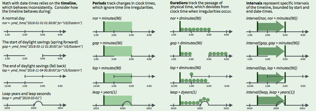
3 ways to represent time spans (From lubridate cheatsheet)

Intervals represent specific intervals of the timeline, bounded by start and end date-times
- Example: People with birthdays between the interval October 23 to November 22 are Scorpios
Periods track changes in clock times, which ignore time line irregularities
- Example: Daylight savings time ends at the beginning of November and we gain an hour - this extra hour is ignored when determining the period between October 23 to November 22
Durations track the passage of physical time, which deviates from clock time when irregularities occur
- Example: Daylight savings time ends at the beginning of November and we gain an hour - this extra hour is added when determining the duration between October 23 to November 22

5.3.1 Time spans using `lubridate`

Using the lubridate package for time spans:

Interval
- Create an interval using interval() or %--%
  - Syntax: interval(<date/time_object1>, <date/time_object2>) or <date/time_object1> %--% <date/time_object2>
Periods
- “Periods are time spans but don’t have a fixed length in seconds, instead they work with ‘human’ times, like days and months.” (From R for Data Science)
- Create periods using functions whose name is the time unit pluralized (e.g., years(), months(), weeks(), days(), hours(), minutes(), seconds())
  - Example: days(1) creates a period of 1 day - it does not matter if this day happened to have an extra hour due to daylight savings ending, since periods do not have a physical length
```
days(1)
#> [1] "1d 0H 0M 0S"
```
- You can add and subtract periods
- You can also use as.period() to get period of an interval
Durations
- Durations keep track of the physical amount of time elapsed, so it is “stored as seconds, the only time unit with a consistent length” (From lubridate cheatsheet)
- Create durations using functions whose name is the time unit prefixed with a d (e.g., dyears(), dweeks(), ddays(), dhours(), dminutes(), dseconds())
  - Example: ddays(1) creates a duration of 86400s, using the standard conversion of 60 seconds in an minute, 60 minutes in an hour, and 24 hours in a day:
```
ddays(1)
#> [1] "86400s (~1 days)"
```
    Notice that the output says this is equivalent to approximately 1 day, since it acknowledges that not all days have 24 hours. In the case of daylight savings, one particular day may have 25 hours, so the duration of that day should be represented as:
```
ddays(1) + dhours(1)
#> [1] "90000s (~1.04 days)"
```
- You can add and subract durations
- You can also use as.duration() to get duration of an interval

Example: Working with interval

# Use `Sys.timezone()` to get timezone for your location (time is midnight by default)
scorpio_start <- ymd("2019-10-23", tz = Sys.timezone())
scorpio_end <- ymd("2019-11-22", tz = Sys.timezone())

scorpio_start
#> [1] "2019-10-23 PDT"
# These datetime objects have class `POSIXct`
class(scorpio_start)
#> [1] "POSIXct" "POSIXt"

# Create interval for the datetimes
scorpio_interval <- scorpio_start %--% scorpio_end  # or `interval(scorpio_start, scorpio_end)`
scorpio_interval <- interval(scorpio_start, scorpio_end)
scorpio_interval
#> [1] 2019-10-23 PDT--2019-11-22 PST

# The object has class `Interval`
class(scorpio_interval)
#> [1] "Interval"
#> attr(,"package")
#> [1] "lubridate"
as.numeric(scorpio_interval)
#> [1] 2595600

Example: Working with period

If we use as.period() to get the period of scorpio_interval, we see that it is a period of 30 days. We do not worry about the extra 1 hour gained due to daylight savings ending:

# Period is 30 days
scorpio_period <- as.period(scorpio_interval)
scorpio_period
#> [1] "30d 0H 0M 0S"

# The object has class `Period`
class(scorpio_period)
#> [1] "Period"
#> attr(,"package")
#> [1] "lubridate"

Because periods work with “human” times like days, it is more intuitive. For example, if we add a period of 30 days to the scorpio_start datetime object, we get the expected end datetime that is 30 days later:

# Start datetime for Scorpio birthdays (time is midnight)
scorpio_start
#> [1] "2019-10-23 PDT"

# After adding 30 day period, we get the expected end datetime (time is midnight)
scorpio_start + days(30)
#> [1] "2019-11-22 PST"

Example: Working with duration

If we use as.duration() to get the duration of scorpio_interval, we see that it is a duration of 2595600 seconds. It takes into account the extra 1 hour gained due to daylight savings ending:

# Duration is 2595600 seconds, which is equivalent to 30 24-hr days + 1 additional hour
scorpio_duration <- as.duration(scorpio_interval)
scorpio_duration
#> [1] "2595600s (~4.29 weeks)"

# The object has class `Duration`
class(scorpio_duration)
#> [1] "Duration"
#> attr(,"package")
#> [1] "lubridate"

# Using the standard 60s/min, 60min/hr, 24hr/day conversion,
# confirm duration is slightly more than 30 "standard" (ie. 24-hr) days
2595600 / (60 * 60 * 24)
#> [1] 30.04167

# Specifically, it is 30 days + 1 hour, if we define a day to have 24 hours
seconds_to_period(scorpio_duration)
#> [1] "30d 1H 0M 0S"

Because durations work with physical time, when we add a duration of 30 days to the scorpio_start datetime object, we do not get the end datetime we’d expect:

# Start datetime for Scorpio birthdays (time is midnight)
scorpio_start
#> [1] "2019-10-23 PDT"

# After adding 30 day duration, we do not get the expected end datetime
# `ddays(30)` adds the number of seconds in 30 standard 24-hr days, but one of the days has 25 hours
scorpio_start + ddays(30)
#> [1] "2019-11-21 23:00:00 PST"

# We need to add the additional 1 hour of physical time that elapsed during this time span
scorpio_start + ddays(30) + dhours(1)
#> [1] "2019-11-22 PST"

6 Appendix

6.1 Special Characters

“A sequence in a string that starts with a \ is called an escape sequence and allows us to include special characters in our strings.”

Credit: Escape sequences from DataCamp

Special characters are characters that will not be interpreted literally.

Common special characters:

\n: newline
\t: tab
\: used for escaping purposes
- \': literal single quote
- \": literal double quote
- \\: literal backslash

These characters followed by a backslash \ take on a new meaning. The n by itself is just an n. When you add a backslash to the \n you are escaping it and making it a special character where \n now represents a newline.

The writeLines() function:

?writeLines

# SYNTAX AND DEFAULT VALUES
writeLines(text, con = stdout(), sep = "\n", useBytes = FALSE)

“writeLines() displays quotes and backslashes as they would be read, rather than as R stores them.” (From writeLines documentation)
When we include escape sequences in the string, it is helpful to use writeLines() to see how the escaped string looks
writeLines() will also output the string without showing the outer pair of double quotes that R uses to store it, so we only see the content of the string

Example: Escaping single quotes

my_string <- 'Escaping single quote \' within single quotes'
my_string
#> [1] "Escaping single quote ' within single quotes"

Alternatively, we could’ve just created the string using double quotes:

my_string <- "Single quote ' within double quotes does not need escaping"
my_string
#> [1] "Single quote ' within double quotes does not need escaping"

Using writeLines() shows us only the content of the string without the outer pair of double quotes that R uses to store strings:

writeLines(my_string)
#> Single quote ' within double quotes does not need escaping

Example: Escaping double quotes

my_string <- "Escaping double quote \" within double quotes"
my_string
#> [1] "Escaping double quote \" within double quotes"

Alternatively, we could’ve just created the string using single quotes:

my_string <- 'Double quote " within single quotes does not need escaping'
my_string
#> [1] "Double quote \" within single quotes does not need escaping"

Notice how the backslash still showed up in the above output to escape our double quote from the outer pair of double quotes that R uses to store the string. This is no longer an issue if we use writeLines() to only show the string content:

writeLines(my_string)
#> Double quote " within single quotes does not need escaping

Example: Escaping double quotes within double quotes

my_string <- "I called my mom and she said \"Echale ganas!\""
my_string
#> [1] "I called my mom and she said \"Echale ganas!\""

Using writeLines() shows us only the content of the string without the backslashes:

writeLines(my_string)
#> I called my mom and she said "Echale ganas!"

Example: Escaping backslashes

To include a literal backslash in the string, we need to escape the backslash with another backslash:

my_string <- "The executable is located in C:\\Program Files\\Git\\bin"
my_string
#> [1] "The executable is located in C:\\Program Files\\Git\\bin"

Use writeLines() to see the escaped string:

writeLines(my_string)
#> The executable is located in C:\Program Files\Git\bin

Example: Other special characters

my_string <- "A\tB\nC\tD"
my_string
#> [1] "A\tB\nC\tD"

Use writeLines() to see the escaped string:

writeLines(my_string)
#> A    B
#> C    D

6.1.1 Escape special characters using Twitter data

Let’s take a look at some tweets from our PAC-12 universities.

Let’s start by grabbing observations 1-3 from the text column.

#Twitter example of \n newline special characters
p12_df$text[1:3]
#> [1] "Big Dez is headed to Indy!\n\n#GoCougs | #NFLDraft2020 | @dadpat7 | @Colts | #NFLCougs https://t.co/NdGsvXnij7"                                                                                                                                                                  
#> [2] "Cougar Cheese. That's it. That's the tweet. 🧀#WSU #GoCougs https://t.co/0OWGvQlRZs"                                                                                                                                                                                             
#> [3] "Darien McLaughlin '19, and her dog, Yuki, went on a #Pullman distance walk this weekend. We will let you judge who was leading the way.🚶‍♀️🐕\n\nTweet a pic of how you are social distancing w/ the hashtag #CougsContain &amp; tag @WSUPullman #GoCougs https://t.co/EltXDy1tPt"

Using writeLines() we can see the contents of the strings as they would be read, rather than as R stores them.

writeLines(p12_df$text[1:3])
#> Big Dez is headed to Indy!
#> 
#> #GoCougs | #NFLDraft2020 | @dadpat7 | @Colts | #NFLCougs https://t.co/NdGsvXnij7
#> Cougar Cheese. That's it. That's the tweet. 🧀#WSU #GoCougs https://t.co/0OWGvQlRZs
#> Darien McLaughlin '19, and her dog, Yuki, went on a #Pullman distance walk this weekend. We will let you judge who was leading the way.🚶‍♀️🐕
#> 
#> Tweet a pic of how you are social distancing w/ the hashtag #CougsContain &amp; tag @WSUPullman #GoCougs https://t.co/EltXDy1tPt

Example: Escaping double quotes using Twitter data

Using Twitter data you may encounter a lot of strings with double quotes.
- In the example below, our string includes special characters \" and \n to escape the double quotes and the newline character.

#Twitter example of \" double quotes special characters
p12_df$text[24]
#> [1] "\"I really am glad that inside Engineering Student Services, I’ve been able to connect with my ESS advisor and professional development advisors there.\"\n-Alexandro Garcia, Civil &amp; Environmental Engineering, 3rd year\n#imaberkeleyengineer #iamberkeley #voicesofberkeleyengineering https://t.co/ToVEynIUWH"

Using writeLines() we can see the contents of the strings as they would be read, rather than as R stores them.
- We no longer see the escaped characters \" or \n

writeLines(p12_df$text[24])
#> "I really am glad that inside Engineering Student Services, I’ve been able to connect with my ESS advisor and professional development advisors there."
#> -Alexandro Garcia, Civil &amp; Environmental Engineering, 3rd year
#> #imaberkeleyengineer #iamberkeley #voicesofberkeleyengineering https://t.co/ToVEynIUWH

Introduction to strings, dates, and time

EDUC 260A: Managing and Manipulating Data Using R

1 Introduction

1.1 Dataset we will use

2 Data structures and types

2.1 Atomtic vectors

2.2 Lists

2.2.1 Dataframes

2.3 Converting between types

3 String basics

4 `stringr` package

4.1 `str_length()`

4.2 `str_c()`

4.3 `str_sub()`

4.4 Other `stringr` functions

5 Dates and times

5.1 Creating date/time objects

5.1.1 Creating date/time objects by parsing input

5.1.2 Creating date/time objects from individual components

5.2 Date/time object components

5.3 Time spans

5.3.1 Time spans using `lubridate`

6 Appendix

6.1 Special Characters

6.1.1 Escape special characters using Twitter data

Introduction to strings, dates, and time

EDUC 260A: Managing and Manipulating Data Using R

1 Introduction

1.1 Dataset we will use

2 Data structures and types

2.1 Atomtic vectors

2.2 Lists

2.2.1 Dataframes

2.3 Converting between types

3 String basics

4 stringr package

4.1 str_length()

4.2 str_c()

4.3 str_sub()

4.4 Other stringr functions

5 Dates and times

5.1 Creating date/time objects

5.1.1 Creating date/time objects by parsing input

5.1.2 Creating date/time objects from individual components

5.2 Date/time object components

5.3 Time spans

5.3.1 Time spans using lubridate

6 Appendix

6.1 Special Characters

6.1.1 Escape special characters using Twitter data

4 `stringr` package

4.1 `str_length()`

4.2 `str_c()`

4.3 `str_sub()`

4.4 Other `stringr` functions

5.3.1 Time spans using `lubridate`